Many lines separate two classes. A support vector machine picks a specific one: the line with the widest possible empty corridor either side of it.
The margin
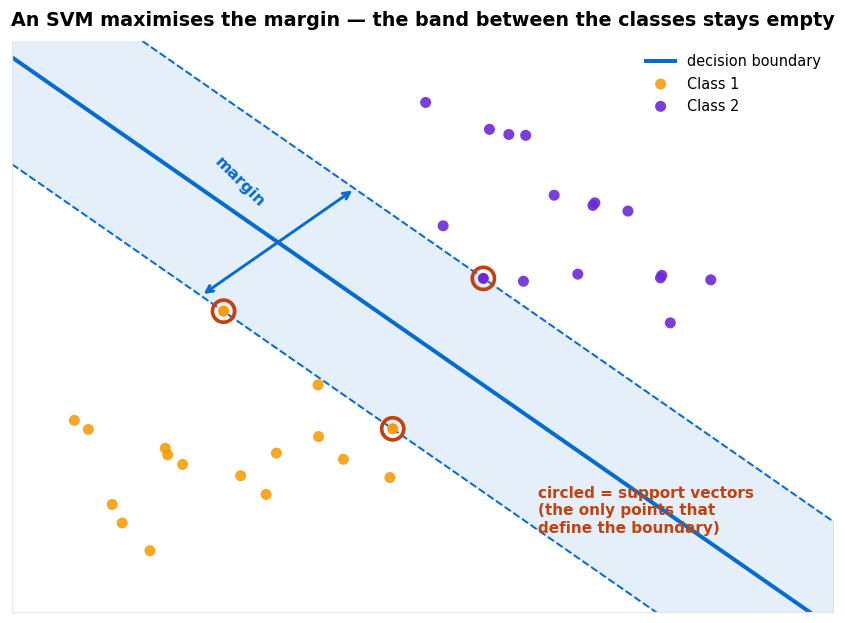
A wide margin means the boundary sits confidently between the classes rather than skimming one of them. That gives a better chance of getting new, slightly different points right — which is the whole aim.
Soft margins and the C parameter
Real data overlaps, so a perfectly empty margin often does not exist. SVMs allow violations and charge for them, with C setting the price.
| C value | Behaviour | Risk |
|---|---|---|
| Small C | Violations are cheap — wide margin, some points inside | Underfitting |
| Large C | Violations are expensive — narrow margin, contorts to fit | Overfitting |
C is the inverse of regularisation strength — small C means heavy regularisation. Tune it on a log scale with cross-validation.
The loss function behind this is hinge loss: zero for points safely outside the margin, growing linearly for those inside or misclassified.
The kernel trick
A straight line cannot separate every dataset. Picture one class in a circle at the centre and the other surrounding it — no line works.
🧪 Lifting the problem into another dimension
The trick: the SVM’s maths only ever needs dot products between points, never the points’ coordinates themselves. A kernel function computes what the dot product would be in the higher-dimensional space — without ever constructing it.
So you get the benefit of a space with thousands of dimensions at the cost of a simple function on the original ones.
Linear for text and high-dimensional data. RBF for everything else — it is the default and handles curved boundaries well, with gamma controlling how tightly the boundary wraps the data. Polynomial exists but is rarely the best choice.
Scale your features, without exception
⚠️ SVMs are defined by distance
Standardise every feature first. This is the most common reason a beginner’s SVM underperforms.
When to use one
SVMs are strong on small to medium datasets with clear separation, and on high-dimensional data such as text — where having more features than samples is fine.
They are a poor fit for very large datasets, because training scales roughly quadratically with the number of rows. Beyond about 100,000 rows, use gradient boosting or a linear model instead.
They also give no natural probability output — the probability=True option fits a separate calibration step and slows training considerably. If you need calibrated probabilities, logistic regression is a better starting point.
🔑 Key Takeaways
- An SVM chooses the boundary with the widest empty margin between the classes.
- Only the support vectors matter — all other training points could be deleted.
Ctrades margin width against violations; small C regularises more.- The kernel trick gives curved boundaries by computing dot products in a space it never builds.
- Scaling is mandatory, and SVMs do not scale well past ~100,000 rows.
Further reading
scikit-learn’s SVM guide covers kernels, the C and gamma parameters and the scaling requirement, and its RBF parameters example shows visually what tuning the two together does to the boundary.
Where to go next
- Naive Bayes — the next algorithm in this sequence
- Hinge loss — the loss function an SVM minimises
- Feature scaling — required before any SVM
- Start Here — the full learning path