A Taylor series rewrites almost any smooth function as an infinite sum of polynomial terms built from its derivatives at a single point — turning hard functions like $e^x$, $\sin x$, and $\ln x$ into simple polynomials you can actually compute.
What is a Taylor series?
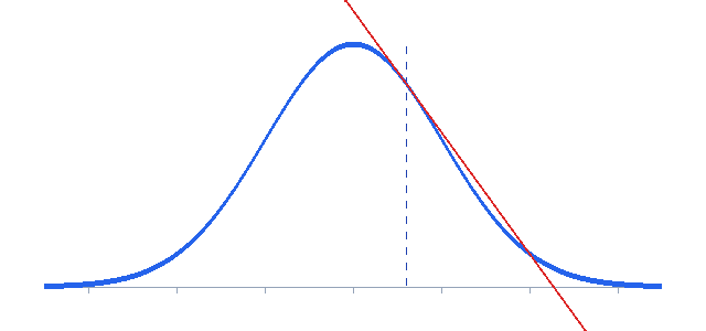
The core idea behind the Taylor series is surprisingly visual: any smooth curve looks like a straight line if you zoom in far enough, and like a parabola if you zoom in a little less. Keep adding higher-power terms and the polynomial bends to match the curve more and more closely. A Taylor series is the exact recipe for that matching polynomial — it reproduces a function’s value, its slope, its curvature, and every higher derivative at one chosen point, called the center.
This is why your calculator can find $\sin(0.5)$ or $e^{1.3}$ at all: under the hood it sums a handful of Taylor terms. It is also why Taylor series sit at the heart of physics approximations and machine-learning optimizers.
If you can differentiate a function, you can approximate it with a polynomial — and the Taylor series tells you exactly which polynomial.
The Taylor series formula
For a function $f$ that is infinitely differentiable at a center $a$:
$$f(x)=\sum_{n=0}^{\infty}\frac{f^{(n)}(a)}{n!}(x-a)^n = f(a) + f'(a)(x-a) + \frac{f”(a)}{2!}(x-a)^2 + \frac{f”'(a)}{3!}(x-a)^3 + \cdots$$Reading it piece by piece:
- $f^{(n)}(a)$ is the $n$-th derivative of $f$ evaluated at the center $a$.
- Dividing by $n!$ is the bookkeeping that makes the polynomial’s $n$-th derivative match the function’s $n$-th derivative.
- The power $(x-a)^n$ measures how far you have moved from the center.
How to find a Taylor series, step by step
- Pick a center $a$. Choose a point near where you need the approximation and where the derivatives are easy to evaluate (use $a=0$ for a Maclaurin series).
- Differentiate repeatedly. Find $f(a), f'(a), f”(a), \dots$ up to the order you want.
- Form each coefficient. Divide the $n$-th derivative value by $n!$ to get the coefficient of $(x-a)^n$.
- Add the terms. Sum them into a polynomial of the chosen order — that is your Taylor approximation.
Prefer to skip the algebra? The free Taylor series calculator does every step and graphs the result.
Worked example 1: the Taylor series of ex
Expand $f(x)=e^x$ about $a=0$. Because every derivative of $e^x$ is $e^x$, and $e^0=1$, every derivative value is $1$:
| n | $f^{(n)}(x)$ | $f^{(n)}(0)$ | coefficient $=f^{(n)}(0)/n!$ |
|---|---|---|---|
| 0 | $e^x$ | 1 | $1$ |
| 1 | $e^x$ | 1 | $1$ |
| 2 | $e^x$ | 1 | $1/2$ |
| 3 | $e^x$ | 1 | $1/6$ |
So $e^x \approx 1 + x + \dfrac{x^2}{2} + \dfrac{x^3}{6} + \dfrac{x^4}{24} + \cdots$ — one of the most useful series in all of mathematics.
Worked example 2: the Taylor series of sin x
The derivatives of $\sin x$ cycle: $\sin x \to \cos x \to -\sin x \to -\cos x \to \sin x \to \cdots$. At $a=0$ that gives $0,1,0,-1,0,1,\dots$, so only the odd powers survive:
$$\sin x \approx x – \frac{x^3}{3!} + \frac{x^5}{5!} – \frac{x^7}{7!} + \cdots$$The matching expansion for cosine keeps only even powers: $\cos x \approx 1 – \frac{x^2}{2!} + \frac{x^4}{4!} – \cdots$
Common Taylor (Maclaurin) series to know
| Function | Series about $a=0$ | Valid for |
|---|---|---|
| $e^x$ | $1 + x + \frac{x^2}{2!} + \frac{x^3}{3!} + \cdots$ | all $x$ |
| $\sin x$ | $x – \frac{x^3}{3!} + \frac{x^5}{5!} – \cdots$ | all $x$ |
| $\cos x$ | $1 – \frac{x^2}{2!} + \frac{x^4}{4!} – \cdots$ | all $x$ |
| $\frac{1}{1-x}$ | $1 + x + x^2 + x^3 + \cdots$ | $|x|<1$ |
| $\ln(1+x)$ | $x – \frac{x^2}{2} + \frac{x^3}{3} – \cdots$ | $-1 < x \le 1$ |
| $(1+x)^p$ | $1 + px + \frac{p(p-1)}{2!}x^2 + \cdots$ | $|x|<1$ |
Choosing the center a
The center is your free choice, and it matters. A Taylor series is sharpest near $a$, so pick a center close to the input you care about and one where the function behaves nicely. Expanding $\ln x$ about $a=1$ (rather than $0$, where it is undefined) is the classic example — the resulting series converges for $0 < x \le 2$.
Why Taylor series matter in machine learning
Beyond calculus class, Taylor series quietly power modern computing:
- Evaluating functions: calculators and CPUs compute $\sin$, $\cos$, and $e^x$ by summing Taylor terms.
- Physics: the small-angle approximation $\sin\theta \approx \theta$ is just the first Taylor term.
- Optimization: gradient descent uses a first-order Taylor approximation of the loss; Newton’s method and second-order optimizers use the quadratic (second-order) one.
🤖 ML insight
Every step of gradient descent assumes that, locally, the loss looks like a straight line; second-order methods assume it looks like a parabola. Both are Taylor approximations — the math on this page is literally the theory behind how neural networks train. Compute the derivatives they need with our derivative calculator.
Frequently asked questions
What is a Taylor series in simple terms?
What is the difference between a Taylor series and a Maclaurin series?
What is the Taylor series formula?
What does the radius of convergence mean?
Why does every term have a factorial?
How is the Taylor series used in machine learning?
Key takeaways
A Taylor series turns hard functions into friendly polynomials built from derivatives at a center, with accuracy that improves with more terms and degrades far from the center. Ready to see it in action? Try the Taylor series calculator, read the Maclaurin series guide, or brush up with the formal Taylor series reference on Wikipedia.