The interquartile range is one of the most useful numbers in statistics, yet it’s often skipped over in favour of the average. This guide explains exactly what the IQR is, how to find it step by step for both odd and even data sets, how it powers outlier detection and box plots, and why it quietly does a lot of work in machine learning.
Key takeaways
- The interquartile range (IQR) is the spread of the middle 50% of your data: $\text{IQR}=Q_3-Q_1$.
- It is robust — outliers barely affect it, unlike the range or the standard deviation.
- It powers the 1.5 × IQR rule for spotting outliers and is the body of every box plot.
- In machine learning it drives robust feature scaling and outlier removal on skewed data.
What is the interquartile range?
The IQR measures how spread out the middle half of a data set is. To get it, you split your ordered data into four equal parts using three cut points called quartiles, then look at the distance between the first and third of those cut points. Everything in between — the central 50% of your values — sits inside the interquartile range.
That “middle 50%” idea is what makes the IQR so valuable. The ordinary range (maximum minus minimum) can be wrecked by a single freak value. The interquartile range ignores the extreme top 25% and bottom 25% entirely, so one ridiculous outlier can’t distort it. For a formal treatment, see the IQR reference.
Quartiles: the building blocks
You can’t understand the IQR without quartiles, so let’s be precise about them. Sort your data from smallest to largest and the quartiles are the three values that chop it into four equally sized groups:
- First quartile (Q1) — the 25th percentile. A quarter of the data lies below it. It is the median of the lower half.
- Second quartile (Q2) — the 50th percentile, which is simply the median. Half the data lies below it.
- Third quartile (Q3) — the 75th percentile. Three quarters of the data lies below it. It is the median of the upper half.
Together with the minimum and maximum, these give the five-number summary (min, Q1, median, Q3, max) — a compact snapshot of any data set. The interquartile range is just the gap between Q1 and Q3 in that summary.
The IQR formula
The formula could not be simpler:
$$\text{IQR}=Q_3-Q_1$$All the real work is in finding Q1 and Q3 correctly. There is a small wrinkle: statisticians use a few slightly different conventions for locating quartiles (the “exclusive” and “inclusive” methods differ in whether the median is included when you split the data). The method below — treating Q1 and Q3 as the medians of the lower and upper halves, excluding the overall median when the count is odd — is the one taught in most courses and used by our median calculator.
How to find the interquartile range step by step
- Sort the data from smallest to largest. Quartiles are meaningless on unordered numbers.
- Find the median (Q2) to split the data into a lower half and an upper half.
- Find Q1 as the median of the lower half, and Q3 as the median of the upper half.
- Subtract: the IQR is $Q_3-Q_1$.
Worked example 1: an odd number of values
Take the data set 7, 2, 9, 4, 12, 5, 8 — seven values.
First, sort it: 2, 4, 5, 7, 8, 9, 12. With seven values the median is the 4th value, 7. Because the count is odd, we set that middle value aside. The lower half is 2, 4, 5 and the upper half is 8, 9, 12.
The median of the lower half is Q1 = 4. The median of the upper half is Q3 = 9. Therefore the interquartile range is:
$$\text{IQR}=Q_3-Q_1=9-4=5$$So the middle 50% of this data set is spread across a range of 5 units. Notice that the largest value, 12, played no part in the calculation — that robustness is the whole point.
Worked example 2: an even number of values
Now take 10, 3, 7, 1, 8, 5 — six values. Sorted: 1, 3, 5, 7, 8, 10. With an even count the data splits straight down the middle into a lower half 1, 3, 5 and an upper half 7, 8, 10.
Q1 is the median of 1, 3, 5, which is 3. Q3 is the median of 7, 8, 10, which is 8. So:
If you ever want to skip the arithmetic, paste either data set into the median calculator — it reports Q1, Q3 and the IQR automatically, which is handy for checking your hand calculations.
The interquartile range and outliers: the 1.5 × IQR rule
The most famous use of the IQR is detecting outliers. A value is flagged as a likely outlier if it falls beyond “fences” placed one and a half interquartile ranges past the quartiles:
$$\text{Lower fence}=Q_1-1.5\times\text{IQR},\qquad \text{Upper fence}=Q_3+1.5\times\text{IQR}$$Anything below the lower fence or above the upper fence is treated as an outlier. Let’s apply it to the first example, where Q1 = 4, Q3 = 9 and IQR = 5. The lower fence is $4-1.5\times5=-3.5$ and the upper fence is $9+1.5\times5=16.5$. Every value in 2, 4, 5, 7, 8, 9, 12 sits comfortably inside that window, so there are no outliers — which matches our intuition.
The box plot connection
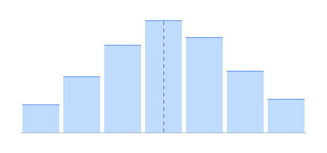
Open any box plot and you are looking at the interquartile range directly. The box stretches from Q1 to Q3, so its length is the IQR. The line inside the box is the median, and the “whiskers” reach out to the most extreme values that still fall inside the 1.5 × IQR fences. Any point beyond a whisker is drawn separately as an outlier. This is why box plots are such an efficient way to compare several groups at a glance: a wide box means a large interquartile range and lots of spread; a narrow box means the middle of the data is tightly packed.
The IQR turns a messy column of numbers into a single, outlier-proof measure of how spread out the typical values really are.
Interquartile range vs range vs standard deviation
Three measures describe spread, and choosing the right one matters. Here is how they compare:
| Measure | What it captures | Affected by outliers? | Best for |
|---|---|---|---|
| Range | Max − min (full spread) | Extremely — one value sets it | Quick, rough idea |
| Interquartile range | Spread of the middle 50% | Barely — ignores the tails | Skewed data, outlier detection |
| Standard deviation | Average distance from the mean | Yes — squares the deviations | Roughly symmetric data |
The rule of thumb: report the median and interquartile range when your data is skewed or full of outliers, and the mean and variance or standard deviation when it is roughly symmetric. House prices and incomes, which have long right tails, are almost always summarised with the median and the IQR for exactly this reason.
Why the interquartile range matters in machine learning
The IQR earns its place in any machine learning toolkit, and it shows up in three practical ways. First, robust feature scaling: libraries like scikit-learn include a RobustScaler that centres each feature on its median and scales it by the interquartile range instead of the standard deviation. On data with heavy outliers, this keeps the scaling stable where standard scaling would be dragged around by the extremes.
Second, outlier removal: the 1.5 × IQR rule is one of the simplest, most defensible ways to filter anomalous rows before training. Because the IQR is robust, the very outliers you want to remove don’t inflate the threshold that’s supposed to catch them — a problem that wrecks naive standard-deviation-based filters.
Third, honest data exploration: when you first meet a dataset, plotting the interquartile range for each feature (via box plots) instantly reveals which columns are skewed, which carry outliers, and which need transforming before a model ever sees them.
🤖 ML insight
When a feature is heavily skewed, scaling it by the standard deviation lets a handful of extreme values dominate. Scaling by the IQR instead — the idea behind RobustScaler — keeps the bulk of the data well-behaved, which is why it’s a go-to for real-world, messy features.
Tips for working with the interquartile range
A few practical pointers save a lot of confusion. Always sort first — it is the single most common source of wrong answers. Be consistent about your quartile method; if you compare two datasets, compute their IQRs the same way. And remember that a small interquartile range doesn’t mean “no variation” — it means the middle of the data is tight, while the tails could still be long. Pair the IQR with a box plot whenever you can, so you see the shape, not just the number.
Frequently asked questions
What is the interquartile range in simple terms?
How do you calculate the IQR?
Why is the interquartile range better than the range?
What is the 1.5 × IQR rule?
Is the interquartile range the same as the standard deviation?
When should I use the interquartile range in machine learning?
Interquartile range: summary
The IQR is the spread of the central 50% of a data set, found by subtracting the first quartile from the third. Its great strength is robustness: outliers, which destroy the range and distort the standard deviation, barely touch it. That robustness is exactly why it underpins outlier detection, box plots, and robust scaling in machine learning. Work through the two examples above, try your own numbers in the median calculator, and explore the rest of the foundations in our statistics for machine learning guide.