Most machine learning models are opaque: a set of weights that predict well and explain nothing. A decision tree is the opposite. It makes decisions the way a person would — one question at a time — and you can follow every step.
What a decision tree looks like
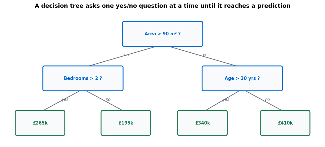
To predict a 120 m² house that is 12 years old: Area > 90? Yes, go right. Age > 30? No, go right again. Predicted price: £410k. That is a complete prediction, and you can explain it to anyone.
How a decision tree chooses its questions
This is the only real algorithm in the whole method. At each node, the tree tries every feature and every possible split point, and asks: which split leaves the two resulting groups most “pure”?
Purity means the group’s outcomes are similar. A group of 20 houses all priced near £200k is pure. A group split evenly between £100k and £500k is not.
| Measure | Used for | Perfectly pure | Worst case |
|---|---|---|---|
| Gini impurity | Classification (the default) | 0 | 0.5 for two classes |
| Entropy | Classification | 0 | 1 for two classes |
| Variance | Regression | 0 | Unbounded |
🧪 Worked example: computing Gini
Gini = 1 − (0.6² + 0.4²) = 1 − (0.36 + 0.16) = 0.48 — close to the worst possible 0.5.
Now split on “contains the word FREE”:
· Yes group: 5 emails, all spam. Gini = 1 − (1.0² + 0²) = 0. Perfectly pure.
· No group: 5 emails, 1 spam, 4 not. Gini = 1 − (0.2² + 0.8²) = 0.32
Weighted average after the split = (5/10 × 0) + (5/10 × 0.32) = 0.16
Impurity fell from 0.48 to 0.16 — a gain of 0.32. The tree tries every candidate split and keeps whichever gives the largest gain.
Then it repeats the whole process on each resulting group, recursively, until it decides to stop.
Knowing when to stop: the overfitting problem
Left alone, a decision tree will keep splitting until every leaf holds a single training example. At that point it is 100% accurate on training data and close to useless on anything new — a textbook case of overfitting.
⚠️ An unrestricted decision tree always overfits
- max_depth — cap how many questions deep the tree can go. The single most effective control.
- min_samples_split — refuse to split a node holding fewer than N examples.
- min_samples_leaf — require every leaf to hold at least N examples.
- Pruning — grow the full tree, then cut back branches that do not help on validation data.
Why beginners should start here
The weaknesses
Instability. Change a few training rows and you can get a visibly different tree. Small data changes flip which split wins at the root, and everything below it changes too.
Axis-aligned splits only. A single decision tree can only cut straight lines parallel to the axes. If the real boundary is diagonal, the tree approximates it with a staircase of many splits — clumsy and prone to overfitting.
Bias toward high-cardinality features. A column with many distinct values offers more possible split points, so it can win by luck. Watch for this if you ever see a tree splitting on something like a customer ID.
🔑 Key Takeaways
- A decision tree asks yes/no questions, choosing each one to maximise the purity of the resulting groups.
- Gini and entropy measure purity for classification; variance does the job for regression.
- An unlimited tree always overfits — control it with max_depth and minimum leaf sizes.
- No feature scaling required, and mixed data types are fine.
- Single trees are unstable; averaging many of them gives a random forest.
Further reading
scikit-learn’s decision trees guide covers the splitting criteria and pruning parameters in full, and its plot_tree function will draw your own trained tree exactly like the diagram above.
Where to go next
- k-nearest neighbours — the next algorithm in this sequence
- Overfitting and underfitting — why depth limits matter
- The confusion matrix — how to evaluate your tree
- Start Here — the full learning path