Understanding the eigenvalues of a 2×2 matrix is a core skill in linear algebra, used everywhere from data science to quantum mechanics. This guide gives you a clear, step-by-step method to find them, with real numbers and expert tips.
What Are Eigenvalues of 2×2 Matrix?
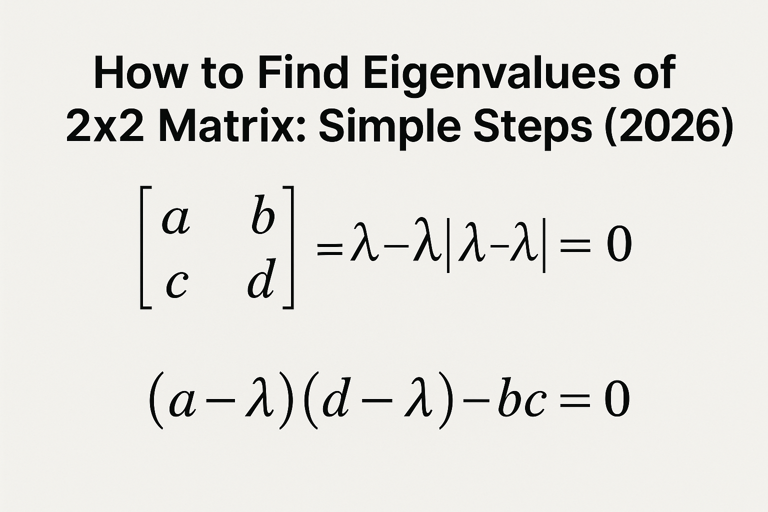
An eigenvalue λ of a square matrix A is a scalar such that Av = λv for some non‑zero vector v (the eigenvector). For a 2×2 matrix, the eigenvalues of 2×2 matrix are found by solving the characteristic polynomial:
$$\det(A – \lambda I) = 0.$$
This expands to $\lambda^2 – \text{tr}(A)\lambda + \det(A) = 0$, where tr(A) is the trace (sum of diagonal entries) and det(A) is the determinant. The two solutions are the eigenvalues of 2×2 matrix. They may be real and distinct, real and repeated, or complex conjugates.
🔑 Key Takeaways
- The eigenvalues of 2×2 matrix are the roots of the characteristic polynomial λ² – (trace)λ + determinant.
- Use the quadratic formula: λ = [tr(A) ± √(tr² – 4det)] / 2.
- The discriminant Δ = tr² – 4det determines whether eigenvalues are real or complex.
- Eigenvectors are not needed to find eigenvalues — the characteristic equation alone suffices.
- Real symmetric 2×2 matrices always have real eigenvalues.
Step‑by‑Step: How to Calculate Eigenvalues of 2×2 Matrix
Follow these four steps every time you need the eigenvalues of a 2×2 matrix. The process works for any 2×2 matrix with real or complex entries.
Add the two diagonal entries: $a_{11} + a_{22}$. This is the coefficient of -λ in the characteristic equation.
For $A = \begin{bmatrix}a & b\\c & d\end{bmatrix}$, $\det(A) = ad – bc$. This is the constant term.
Write $\lambda^2 – \text{tr}(A)\lambda + \det(A) = 0$. This quadratic always holds for the eigenvalues of a 2×2 matrix.
Use $\lambda = \frac{\text{tr}(A) \pm \sqrt{(\text{tr}(A))^2 – 4\det(A)}}{2}$. Simplify to get the two eigenvalues.
That’s it. After a few practice runs, finding the eigenvalues of a 2×2 matrix becomes almost automatic.
Worked Example: Finding Eigenvalues of 2×2 Matrix
Let’s apply the steps to a concrete matrix:
$$A = \begin{bmatrix}2 & 1\\1 & 2\end{bmatrix}$$
Step 1: Trace = $2 + 2 = 4$.
Step 2: Determinant = $(2)(2) – (1)(1) = 4 – 1 = 3$.
Step 3: Characteristic equation: $\lambda^2 – 4\lambda + 3 = 0$.
Step 4: Solve: $\lambda = \frac{4 \pm \sqrt{16 – 12}}{2} = \frac{4 \pm 2}{2}$. So $\lambda_1 = 3$, $\lambda_2 = 1$. The eigenvalues of this 2×2 matrix are 3 and 1.
Check: For λ=3, $A – 3I = \begin{bmatrix}-1 & 1\\1 & -1\end{bmatrix}$ has non‑zero nullspace, confirming the eigenvalue. Notice the eigenvalues in this symmetric example are real and distinct.
🧪 Worked example
Trace = 4+3=7, det=4(3)-2(1)=12-2=10
Equation: λ² – 7λ +10=0 → λ = (7 ± √(49-40))/2 = (7 ± 3)/2 → λ=5, λ=2.
The solutions are 5 and 2.
When Eigenvalues of 2×2 Matrix Are Complex
The discriminant $\Delta = \text{tr}^2 – 4\det$ determines the nature. If $\Delta < 0$, the eigenvalues of a 2x2 matrix are complex conjugates. For example, $A = \begin{bmatrix}0 & -1\\1 & 0\end{bmatrix}$ has trace 0, determinant 1, so $\Delta = -4$. The eigenvalues are $i$ and $-i$, where $i = \sqrt{-1}$.
Complex eigenvalues still satisfy the characteristic equation and appear in conjugate pairs. Many physical systems, such as oscillators, produce complex solutions. For instance, the matrix $A = \begin{bmatrix}1 & -2\\1 & 1\end{bmatrix}$ has trace 2, determinant 3, discriminant -8, yielding eigenvalues $1 \pm i\sqrt{2}$. These complex values indicate oscillatory behavior in differential equations.
When working with complex eigenvalues, remember that the corresponding eigenvectors also come in complex conjugate pairs. The method for finding them remains identical: you still compute $\det(A – \lambda I)=0$. The answer may involve imaginary numbers, which is perfectly valid in linear algebra.
Common Mistakes When Computing Eigenvalues of 2×2 Matrix
Another mistake is miscomputing the determinant, especially when b and c are negative. Double‑check: $\det = ad – bc$, not $ad + bc$. A small sign error changes the eigenvalues completely.
Also, beginners sometimes think the eigenvalues are the diagonal entries themselves. That’s only true for triangular or diagonal matrices. For a general $2\times 2$, the eigenvalues are not simply the diagonal elements. For example, $A = \begin{bmatrix}1 & 2\\0 & 3\end{bmatrix}$ has diagonal entries 1 and 3, yet its eigenvalues are indeed 1 and 3 because it’s triangular. But for $A = \begin{bmatrix}1 & 2\\1 & 3\end{bmatrix}$, the diagonal entries are 1 and 3, but the computed eigenvalues are 4 and -1.
Watch out for arithmetic errors when simplifying the square root. Always compute the discriminant carefully: $\Delta = \text{tr}^2 – 4\det$. If you misplace a sign, your eigenvalues will be off.
“The eigenvalues of a 2×2 matrix are the two numbers that make the matrix shift by exactly λ in every direction. Get them right, and half the rest of linear algebra falls into place.”
At‑a‑Glance Comparison: Real Symmetric vs General 2×2
| Property | Real symmetric 2×2 | General 2×2 (real entries) |
|---|---|---|
| Eigenvalues always real? | Always (Δ ≥ 0) | Maybe real, maybe complex |
| Eigenvectors orthogonal? | Yes | Not generally |
| Formula works | Standard characteristic eqn | Same, but watch for complex results |
| Example | $\begin{bmatrix}1&0\\0&2\end{bmatrix}$ eigenvalues 1,2 | $\begin{bmatrix}0&-1\\1&0\end{bmatrix}$ eigenvalues i, -i |
This table highlights key differences. Regardless, the method to find the eigenvalues of a 2×2 matrix is identical in both cases.
Pros and Cons of the Characteristic Equation Method
✅ Pros
- Always works for 2×2 matrices
- Only requires trace and determinant
- Gives both eigenvalues at once
- No need to compute eigenvectors
- Works for real and complex entries
❌ Cons
- Can involve square roots of negatives
- Doesn’t directly give eigenvectors
- May be less efficient for larger matrices
- Requires careful handling of arithmetic
Applications That Depend on Eigenvalues of 2×2 Matrix
Eigenvalues of a 2×2 matrix appear in hundreds of real‑world contexts. Here are a few:
- Image processing: The 2×2 structure tensor at each pixel has eigenvalues that indicate edge strength and orientation.
- Differential equations: The stability of a 2×2 linear system is determined by the eigenvalues of its matrix — negative real parts mean stability.
- Game theory: Payoff matrices in 2×2 games have eigenvalues related to mixed Nash equilibria.
- Machine learning: Principal component analysis (PCA) often reduces to eigenvalue problems for 2×2 covariance matrices when working with two features.
In each case, computing the eigenvalues quickly and accurately is essential.
Related Concepts: Deepen Your Understanding
Once you master the eigenvalues of a 2×2 matrix, explore these natural next steps:
- Eigenvectors and eigenvalues explained with practical examples — pairs eigenvectors with eigenvalues for a complete picture.
- Determinant of a matrix calculator and guide — master determinants, a key ingredient in the characteristic equation.
- 2×2 identity matrix: definition and properties — understand how the identity interacts with eigenvalue problems.
These resources build directly on the eigenvalues of a 2×2 matrix and will help you see the bigger picture.
For further reading, Wikipedia’s article on eigenvalues and eigenvectors provides a comprehensive mathematical treatment, and ▶ Watch related videos on YouTube for step‑by‑step visual tutorials.
Frequently Asked Questions
What is the formula for eigenvalues of a 2×2 matrix?+
Can a 2×2 matrix have complex eigenvalues?+
How do I check if my eigenvalues are correct?+
Are the eigenvalues always the diagonal entries?+
What does it mean when a 2×2 matrix has repeated eigenvalues?+
We hope this guide has made finding the eigenvalues of a 2×2 matrix straightforward and reliable. Practice with a few different matrices — including symmetric, non-symmetric, and those with complex eigenvalues — and you will soon handle them with confidence.