Hinge loss is the objective behind support vector machines, and it thinks about classification differently from probability-based losses. Instead of asking “what probability did you give the right class?” it asks “did you get the answer right, and with enough margin to be safe?” It gives zero penalty to confident correct predictions and a linearly growing penalty to everything else, which is what produces the wide, robust decision boundaries SVMs are famous for.
What is hinge loss?
Hinge loss works with labels written as −1 and +1 rather than 0 and 1, and with a raw model score rather than a probability. It multiplies the label by the score to get the margin: a positive margin means the prediction is on the correct side, a negative margin means it is wrong. The loss is zero as soon as that margin reaches 1 — correct and confident — and it rises in a straight line as the margin drops below 1. So hinge loss does not merely want correct answers; it wants them with room to spare, and it stops caring the moment that comfortable margin is achieved.
That “stop caring once you are safe” behaviour is what separates it from cross-entropy, which keeps nudging even correct, confident predictions toward ever-higher probability.
The hinge loss formula
Here y is the true label (−1 or +1) and ŷ is the raw score. The product y·ŷ is the margin. When the margin is at least 1 the expression inside is zero or negative, so the hinge loss is 0; when the margin is below 1 — including every misclassification — the loss grows linearly. The “1” is the target margin, and it is what pushes the SVM to separate the classes by the widest possible gap.
See it: hinge loss vs the margin
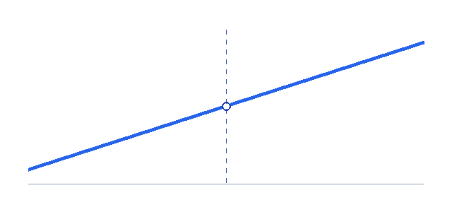
The blue line is the penalty as the margin changes. It sits flat at zero to the right (correct and confident), then kicks up in a straight line once the margin drops below 1 — the “hinge” that gives the loss its name.
Why the margin matters
A worked example
Take a true label of +1 and three different model scores. The margin equals the score here, and the penalty follows directly:
A score of +2 is correct with margin to spare, so the loss is zero. A score of +0.5 is correct but inside the margin, so it still pays 0.5. And a wrong score of −1 pays 2. The lesson: being right is not enough — the loss wants you to be right convincingly.
Hinge loss vs cross-entropy
| Aspect | the loss | Cross-entropy |
|---|---|---|
| Works on | raw scores, ±1 labels | probabilities, 0/1 labels |
| Outputs probabilities? | no | yes |
| Penalty once correct | zero past the margin | never quite zero |
| Classic home | SVMs | neural networks |
If you need calibrated probabilities, use cross-entropy. If you only need a decisive boundary and value robustness, the loss is a natural fit.
Common mistakes to avoid
Hinge loss in Python
import numpy as np

def hinge(y, score):     # y in {-1, +1}
    return np.maximum(0, 1 - y * score).mean()

y = np.array([1, -1, 1]); s = np.array([2.0, -0.5, 0.3])
print(hinge(y, s))       # 0.23
Scikit-learn uses it in LinearSVC and SGDClassifier(loss="hinge"); the squared variant is squared_hinge. See the Wikipedia the loss article for more.
Putting it into practice
the loss shows up most in linear support vector machines and in large-margin variants of other models, and it pairs naturally with L2 regularisation, which together set the width of the margin. A common squared version squares the penalty so that violations grow quadratically, giving a smoother objective at the cost of more sensitivity to outliers. If you are training deep networks you will usually prefer cross-entropy for its probabilities and smooth gradient, but the loss remains a clean, interpretable choice whenever the goal is simply a confident, well-separated boundary rather than a calibrated probability. As always, match your label encoding to the loss — the single most common reason a the loss model fails to learn is labels left as 0 and 1 instead of the −1 and +1 the margin formula expects.
The squared variant and smoothness
There is a popular squared version that squares the penalty instead of growing it linearly, which makes the objective smooth everywhere and easier for gradient methods to optimise, at the price of caring more about the worst violations. The trade-off mirrors the one between absolute and squared error in regression: the plain version is more robust to outliers, while the squared version converges more smoothly but chases extreme points harder. Both share the defining feature of demanding a margin rather than mere correctness, and both ignore points that are already safely on the right side. Choosing between them is usually an empirical question — try both and keep whichever validates better — but the squared form is a sensible default when you want the margin idea together with a gradient that does not have a sharp kink.
Where the margin idea lives today
Although support vector machines are no longer the first tool most people reach for, the margin idea behind them is very much alive. Large-margin objectives appear in metric learning, where models are trained so that similar items sit closer together than dissimilar ones by a fixed gap, and in ranking systems that want the correct item scored above the rest by a comfortable distance. The same “be right, and be right with room to spare” principle shows up in triplet and contrastive objectives that power face recognition and modern retrieval. So even if you never train a classic support vector machine, understanding the margin gives you a mental model that transfers directly to a whole family of modern techniques, and it is a useful counterpoint to the probability-first thinking that dominates deep learning.
Strengths, limits, and when to reach for it
The biggest practical strength is decisiveness: because the penalty vanishes once a point is safely classified, the trained model concentrates entirely on the difficult cases near the boundary, which often gives clean, robust separation on well-structured data. The flip side is that it hands you no probabilities, only scores, so any time you need a calibrated confidence — for ranking by likelihood, for thresholding against a business cost, or for combining models — you must calibrate separately or choose a probability-based objective instead. It also assumes the classes are more or less separable; on very noisy, heavily overlapping data the margin idea has less to offer than a probabilistic approach. A good rule of thumb is to reach for it when you want a crisp linear boundary with strong generalisation and do not need probabilities, and to prefer a log-based objective when calibrated confidence is part of the deliverable. It also rewards good feature engineering more visibly than probabilistic objectives do: because it only cares about the points near the boundary, giving the model features that separate those hard cases cleanly tends to translate into an immediately wider, more confident margin. That makes it a satisfying teaching tool, since the effect of a better feature or a stronger regulariser shows up directly in how far the boundary sits from the nearest examples.