The softmax function is how a neural network turns a handful of raw scores into class probabilities that add up to 100%. It is the standard final layer for single-label multi-class classification — deciding which one of ten digits, or one of a thousand ImageNet classes, an input belongs to. This guide covers the softmax function’s formula, a numerical-stability trick, softmax versus sigmoid, and Python code.
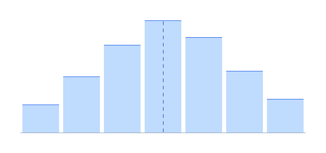
Try it: interactive softmax calculator
Change the three logits and watch the softmax function convert them into probabilities that always sum to 100%.
Enter three logits (raw scores) — softmax turns them into probabilities that sum to 100%:
The softmax function formula
The softmax function takes a vector of raw scores (logits) and returns a probability distribution: each output is between 0 and 1, and all outputs sum to exactly 1. The exponential exaggerates differences, so the largest logit dominates — but softly, keeping some probability on the runners-up.
Why subtract the max?
Softmax vs sigmoid
A sigmoid squashes one number independently; the softmax function couples several numbers so they compete and sum to 1. Use sigmoid for binary or multi-label output, and the softmax function for single-label multi-class output. See the full comparison in sigmoid vs softmax.
Softmax and cross-entropy
The softmax function is almost always paired with the cross-entropy loss for classification. Together they yield a clean gradient (predicted probability minus true label), which is why the pairing is the default final layer of classification networks.
Softmax function in Python
import numpy as np

def softmax(z):
    z = z - np.max(z)          # numerical stability
    e = np.exp(z)
    return e / e.sum()

print(softmax(np.array([2.0, 1.0, 0.1])))
# [0.659 0.242 0.099]
More detail is in the Wikipedia softmax article.
Temperature and confidence
A single extra knob, called temperature, reshapes the output in a way that is worth understanding. Dividing the scores by a value greater than one before normalising flattens the distribution, spreading probability more evenly and making the model less confident; dividing by a value below one sharpens it toward a near-one-hot spike. At training time this is the mechanism behind knowledge distillation, where a large model’s softened outputs teach a smaller one far more than hard labels could, because the soft distribution reveals how the big model rates the runner-up classes. At inference time, tuning temperature is a cheap way to calibrate an over-confident model so its stated probabilities better match how often it is actually right. The same normalisation you use every day, with one small change, becomes a tool for both compression and calibration.
Where it powers modern models
Its reach goes far beyond the final classification layer. The attention mechanism at the heart of every transformer uses it to turn raw compatibility scores between tokens into a set of weights that sum to one, deciding how much each token should attend to every other. Reinforcement-learning policies use it to convert action scores into a probability distribution the agent samples from. Anywhere a model must turn a vector of arbitrary scores into a competing set of choices, this is the tool doing the work, which makes it one of the most quietly ubiquitous operations in all of deep learning. Recognising it in these different settings helps you read architectures: wherever you see scores becoming a distribution that sums to one, the same idea is at play.
The stability trick, in depth
Because it exponentiates its inputs, a large score can overflow to infinity and wreck the result, so every serious implementation first subtracts the maximum score from all of them. This shift leaves the output mathematically unchanged — the constant cancels in the ratio — while guaranteeing the largest exponent is exactly one and the rest are smaller, which never overflows. It is a tiny detail with outsized importance, and it is the main reason frameworks prefer to fuse the operation with the loss and ask for raw scores: the fused path applies the shift for you and avoids ever materialising the dangerous intermediate probabilities. Anyone writing a custom version should copy this trick verbatim.
Argmax, sampling, and reading the output
Once you have a distribution, there is more than one way to use it. Taking the highest-probability class — argmax — is the standard choice for a single confident prediction, but it throws away all the nuance in the runner-up probabilities. Sampling from the distribution instead introduces controlled randomness, which is exactly what text generators do to produce varied, natural output rather than the same deterministic answer every time. And keeping the full distribution lets downstream code reason about uncertainty, combine models, or apply a custom decision threshold. Choosing among these is a modelling decision in its own right, separate from the network that produced the scores, and getting it right is often the difference between a system that feels rigid and one that feels natural.
Pitfalls that trip up beginners
Several recurring mistakes are worth naming so you can avoid them. The first is the double-normalisation bug: applying the transform yourself and then handing the probabilities to a loss that applies it again, which silently flattens the gradient and hobbles training. The second is confusing it with a simple element-wise squashing function — it is not; every output depends on every input, because the denominator sums over the whole vector, so you cannot compute one output in isolation. The third is expecting it to fix class imbalance; it only converts scores to probabilities and does nothing about a skewed dataset, which still needs weighting or resampling. A fourth is reading a high top probability as calibrated confidence when the model has never been calibrated — a network can output 0.99 and still be wrong far more than one percent of the time. Keeping these four traps in mind, and remembering that the operation always couples the classes so they compete and sum to one, will steer you clear of the subtle bugs that most often make a classifier behave strangely despite looking correct on the surface.
From logits to a final decision
It helps to trace the whole journey once, end to end, because seeing it as a pipeline dissolves most of the confusion beginners feel. The network’s last linear layer produces a vector of raw scores, one per class, that can be any real number, positive or negative, large or small. Those scores mean nothing on their own; they are just relative preferences. The normalising step exponentiates each, which makes them all positive and stretches the gaps so a modestly higher score becomes a noticeably higher weight, then divides by the total so the whole vector sums to one and can be read as a probability distribution. At that point you finally have something interpretable: a confidence for every class that competes against the others. During training, a log-based loss compares that distribution against the true label and sends back a gradient that nudges the scores so the correct class gets a larger share next time. At inference you collapse the distribution into an action — usually by taking the most probable class, sometimes by sampling, sometimes by thresholding against a business cost. Every stage has a clear job: the linear layer proposes, the exponential-and-normalise step turns proposals into competing probabilities, the loss teaches, and the decision rule acts. Once you can narrate those four steps without hesitation, the operation stops being a mysterious black box and becomes the obvious, almost inevitable way to turn a pile of raw scores into a confident, trainable choice among classes.
A common beginner mistake
A frequent error is applying the transform twice — once inside the model and again inside the loss. Most deep-learning libraries expect raw logits in their cross-entropy loss and apply the exponential normalisation internally for numerical stability, so adding your own on top double-counts it and quietly hurts training. When in doubt, pass logits to the loss and apply the normalisation explicitly only when you actually need probabilities for display or thresholding. A second subtlety is temperature: dividing the logits by a value greater than one before normalising produces softer, less confident distributions, which is useful for knowledge distillation and for calibrating over-confident models. Reading your framework’s documentation on these two details — where normalisation happens and how temperature is applied — saves hours of confused debugging and mysteriously bad accuracy.
Related activation functions
- Activation Functions — the complete guide (hub).
- Sigmoid Function — the binary-output version.
- Sigmoid vs Softmax — the decision guide.
- Classification Metrics — scoring the outputs.