The sigmoid function is the classic S-shaped curve that squashes any real number into a value between 0 and 1. For decades it was the default activation in neural networks, and it is still the standard choice for the output of a binary classifier and the engine inside logistic regression. This guide covers the sigmoid function’s formula, derivative, its vanishing-gradient weakness, and working Python code.
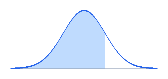
Try it: interactive sigmoid plot
The blue curve is the sigmoid function; the orange dashed curve is its derivative, which peaks at just 0.25 — the seed of the vanishing-gradient problem.
The sigmoid function formula
The sigmoid function (also called the logistic function) maps every real number to the open interval (0, 1). Large positive inputs approach 1, large negative inputs approach 0, and σ(0) = 0.5. That bounded, probability-like output is why the sigmoid function is the natural choice for the output neuron of a binary classifier.
The derivative of the sigmoid function
This elegant self-referential derivative makes backpropagation cheap. But notice its maximum value is only 0.25 (at x = 0) and it falls toward zero in both tails.
Where to use the sigmoid function
The sigmoid function is also the link function in logistic regression, turning a linear score into a probability.
Sigmoid function in Python
import numpy as np

def sigmoid(x):
    return 1 / (1 + np.exp(-x))

def sigmoid_derivative(x):
    s = sigmoid(x)
    return s * (1 - s)

print(sigmoid(np.array([-4.0, 0.0, 4.0])))
# [0.018 0.5   0.982]
See the Wikipedia logistic function article for the full derivation.
Its role in logistic regression
Long before neural networks, the same S-shaped curve was the heart of logistic regression, the workhorse of classical statistics for modelling probabilities. There it maps a linear combination of features onto a value between zero and one that is read directly as the probability of the positive class, and fitting the model means finding the weights that make the observed labels most likely. That lineage is why the curve feels so natural at the output of a modern binary classifier: a single neuron applying it turns the network’s raw score into exactly the calibrated probability logistic regression was designed to produce. Understanding this connection also demystifies why the pairing with a log-based loss is so standard — it is the same maximum-likelihood recipe statisticians have used for a century, now sitting on top of a deep network instead of a linear model.
The saturation story in detail
The curve’s defining weakness is saturation. For inputs beyond roughly plus or minus five it flattens almost completely, so its slope — and therefore the gradient that flows back through it — falls to nearly zero. In a shallow model that barely matters, but stack several such layers and the tiny slopes multiply together, shrinking the learning signal toward nothing by the time it reaches the early layers. That compounding is the mechanism behind the vanishing-gradient problem that stalled deep learning for years, and it is the single reason the curve was displaced from hidden layers by the rectified family. Seeing the mechanism clearly also tells you when the curve is still safe to use: at the output, where there is no deeper layer for its small gradient to starve.
Numerical stability in code
A naive implementation can overflow: exponentiating a large negative input produces a huge number and can return a not-a-number result. Mature libraries avoid this by computing the function in two branches depending on the sign of the input, or by fusing it directly into the loss so the risky intermediate value never appears. This is why frameworks encourage you to hand the loss your raw scores and let it apply the curve internally rather than doing it yourself — the fused version is both faster and numerically safe. If you ever implement it by hand for a custom layer, clamp the input to a sensible range or use the standard stable formulation, and you will avoid a class of silent training failures that are otherwise maddening to track down.
How it compares to its alternatives
Set beside its relatives, the curve occupies a clear niche. Its zero-to-one range makes it the natural choice for a probability output and for the gates inside recurrent units, where a value that means “how much to let through” is exactly what is wanted. Against the hyperbolic tangent it loses for hidden layers because it is not zero-centred and has a shallower peak gradient, and against the rectified family it loses badly on depth because of saturation. Knowing these trade-offs turns the choice into a quick decision: reach for it at the output of a binary model or inside a gate, and reach for a rectifier almost everywhere else.
Inside recurrent gates
One place the curve remains genuinely irreplaceable is inside the gates of recurrent units such as LSTM and GRU cells. There, its job is not to be a general non-linearity but to act as a soft switch: a value near zero means “block this signal” and a value near one means “let it through,” with a smooth range in between that the network can tune. Because the output is bounded firmly between zero and one, it can never blow up the cell state it controls, no matter how long the sequence runs, which is exactly the stability a recurrent loop needs. The hyperbolic tangent handles the candidate values that flow through those gates, while the zero-to-one curve handles the gating itself — a division of labour that has survived every attempt to simplify these cells. So even in an era dominated by transformers, anyone working with recurrent models meets the curve daily, and understanding its bounded, saturating shape is the key to understanding how a gate decides what to remember and what to forget.
A worked intuition
Put a concrete number through the curve and its behaviour stops feeling abstract. An input of zero comes out as exactly one-half, the point of maximum steepness, where a small change in the input moves the output the most and learning is fastest. Push the input up to two and the output climbs to about 0.88; push it to four and it reaches roughly 0.98; by six it is essentially one and barely moves however hard you push, which is saturation in action. The negative side mirrors this exactly: minus two gives about 0.12, minus four about 0.02, and beyond that the output is pinned near zero. Notice how the interesting, responsive region is narrow — roughly between minus three and plus three — and everything outside it is nearly flat. That single fact drives almost every practical rule of thumb about the curve: why inputs should be scaled to sit in that responsive band, why a poorly initialised network whose pre-activations start large will barely learn, and why stacking many of these units drains the gradient so quickly. Once you can picture those numbers, you can predict how a unit will behave in any situation without reaching for the formula, and the earlier discussion of saturation and vanishing gradients becomes something you can feel rather than merely recite.
A brief history
The underlying logistic curve dates back to 19th-century population studies by Pierre François Verhulst, long before neural networks existed. It entered machine learning through logistic regression, then became the standard neuron output in the perceptron and the multilayer networks of the 1980s and 1990s. Its retreat from hidden layers came only around 2012, when researchers realised that deeper models needed activations whose gradients did not fade with depth. Today it survives mainly at the output, where a bounded value between zero and one is exactly what a probability needs, and as a teaching tool for understanding why non-linearity matters at all. Understanding this one curve makes every other activation easier to reason about, because most of them are described by how they improve on its two weaknesses: saturation and a non-zero-centred output.
Related activation functions
- Activation Functions — the complete guide (hub).
- Softmax Function — sigmoid’s multi-class cousin.
- Tanh — the zero-centred alternative.
- Sigmoid vs Softmax — which to use when.