Diffusion Models Explained: How AI Turns Noise Into Images

Most of the AI image generators you have heard of, including Stable Diffusion, DALL·E 2 and 3, and Google’s Imagen, are built on diffusion models. The core idea is surprisingly simple, and it comes down to one trick: destroying an image is easy, so train a network to reverse the destruction a tiny piece at a time.

The forward process: add noise until nothing is left

Take a training image and add a small amount of random Gaussian noise to every pixel. Then do it again, and again. After enough steps the picture is gone and what remains is indistinguishable from pure static. This is the forward process, and it involves no learning at all. It is a fixed recipe.

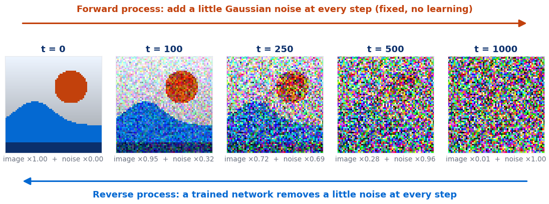
The original DDPM paper (Ho et al., 2020) used 1,000 steps. The noise added at each step is tiny, starting at a variance of 0.0001 and rising to 0.02. The figure uses exactly that schedule. Pixel values are scaled to the range −1 to 1, and the numbers under each frame show how much of the original image and how much noise make up that frame.

One helpful fact makes training practical. Because each step just adds more normally distributed noise, you don’t have to run 500 steps to reach step 500. There is a closed-form shortcut:

noisy image at step t = √ᾱt × original + √(1 − ᾱt) × noise

Here ᾱ_t (“alpha-bar”) is a number that falls from 1 towards 0 as t grows. At t = 250 it is 0.52, so the frame is 0.72 × image + 0.69 × noise. At t = 500 it is 0.079: 0.28 × image + 0.96 × noise. By t = 1000 the image weight is 0.006, effectively zero.

The reverse process: train a network to undo one step

Going forward is trivial. Going backward, from static to a sharp image, is the hard part, and it is what the neural network learns. Rather than predicting the clean image directly, the standard approach asks the network a simpler question: given this noisy image and the step number t, what noise was added? If you know the noise, you can subtract a little of it and move one step closer to a clean image.

The network is usually a U-Net, a convolutional network that shrinks the image down to capture overall layout and then expands it back to full resolution, with shortcuts that keep fine detail. Newer models increasingly replace it with a transformer. Either way, the step number t is fed in too, because removing noise from a nearly clean image is a very different job from finding structure in near-static.

Generating an image from pure noise

Once trained, generation runs the film backwards:

1. Start with pure random noise, the same shape as an image.
2. Ask the network to predict the noise in it at step t = 1000.
3. Remove a portion of that predicted noise (and, in the original method, add back a little fresh randomness), giving a slightly cleaner image for step 999.
4. Repeat all the way down to step 0.

Early steps settle the rough composition, such as where the bright blob and the dark mass go. Later steps add edges, texture and fine detail. Every run starts from different random noise, so every run produces a different image.

Text conditioning in plain words

So far the model makes an image, not the image you asked for. To steer it with a prompt, the text is first turned into a sequence of vectors by a text encoder. Stable Diffusion 1.x used the text half of CLIP, a model trained to match captions with pictures. Those embeddings are passed into the denoising network at every step through cross-attention, so each region of the image being denoised can “look at” the words most relevant to it. The question becomes: what noise was added, given that this is meant to be a red fox in snow?

On its own that conditioning tends to be weak, so almost every system uses classifier-free guidance. At each step the network makes two predictions: one with the prompt and one without. The difference between them points in the “more like the prompt” direction, and the sampler exaggerates it. A guidance scale of about 7 is a common default. Higher values follow the prompt more literally, and too high gives harsh, oversaturated images.

Why diffusion models beat GANs on stability

Before diffusion, the best image generators were GANs (generative adversarial networks): a generator tries to fool a discriminator, which tries to tell real images from fakes. When it works it is fast and sharp, but training is a balancing act between two networks. If one gets ahead, learning stalls or collapses. Mode collapse is the classic failure, where the generator finds a few outputs that fool the discriminator and produces little else.

Diffusion models avoid that fight. Training is a plain regression problem: predict the noise and minimise mean squared error. There is one network, one stable loss function, and a loss curve that goes steadily down. Because the loss covers every training image at every noise level, the model is pushed to cover the full variety of the data rather than a few safe modes. In 2021 Dhariwal and Nichol showed diffusion models beating the best GANs on standard image-quality benchmarks, and the field moved over quickly.

Latent diffusion: how Stable Diffusion made it affordable

Running hundreds of denoising steps on full-resolution pixels is expensive. A 512 × 512 colour image has 786,432 numbers. Latent diffusion (Rombach et al., 2022), the method behind Stable Diffusion, adds a separate autoencoder that compresses the image into a much smaller “latent” grid of 64 × 64 × 4 = 16,384 numbers, 48 times fewer, while keeping what the picture looks like.

The whole diffusion process, both training and generation, happens in that compressed space. Only at the very end does the autoencoder’s decoder turn the finished latent back into pixels. The expensive network works on a grid 48 times smaller at every one of its steps, which is why Stable Diffusion runs on a single consumer graphics card rather than a data centre.

Further reading

The original Denoising Diffusion Probabilistic Models paper (Ho et al., 2020) sets out the noise schedule and training recipe used here, and High-Resolution Image Synthesis with Latent Diffusion Models (Rombach et al., 2022) is the paper behind Stable Diffusion.

Where to go next

• Convolutional neural networks: the building blocks of the U-Net denoiser
• Attention explained: how the prompt reaches every step
• What is a large language model? The other half of generative AI
• Start Here: the full learning path