Everything else in this series works on rows and columns. Images are different, and feeding them to an ordinary neural network fails for a reason worth understanding.
Why ordinary networks fail on images
A modest 200×200 colour image has 120,000 numbers. Connect that to a first hidden layer of 1,000 neurons and you need 120 million weights — in the first layer alone.
⚠️ And it learns the wrong thing
It also throws away the fact that neighbouring pixels are related, because flattening an image into a list destroys the spatial arrangement entirely.
The convolution
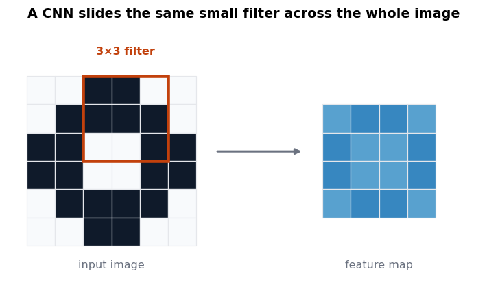
A filter is a small grid of weights — typically 3×3. Place it over a patch of the image, multiply each weight by the pixel beneath it, sum the results. That is a dot product, and it produces one number saying how strongly this patch matches the filter’s pattern.
Slide the filter across the whole image and you get a feature map: a picture of where that pattern occurs.
That 3×3 filter has nine weights. The fully connected layer needed 120 million.
What the filters learn
Nobody designs them. They are weights, learned by backpropagation exactly like any others. What is striking is how consistently a hierarchy emerges:
Each layer composes what the previous one found, which is exactly the argument for depth made in the neural network post — here you can actually see it happening.
Pooling and the rest of the architecture
Pooling shrinks the feature maps, usually by taking the maximum of each 2×2 block. This cuts computation and adds a little tolerance to small shifts — a feature detected one pixel over still survives.
A typical CNN alternates convolution, ReLU and pooling several times, then flattens the result into a few ordinary dense layers and a softmax output. The convolutional part extracts features; the dense part classifies them.
Two things that matter more than architecture
Data augmentation. Randomly flip, rotate, crop and adjust the brightness of your training images. Each variation is effectively a new example, and it teaches the network that a rotated cat is still a cat. It is the most effective single defence against overfitting in vision.
🧪 Transfer learning: do not train from scratch
So take a network already trained on millions of images, freeze those early layers, and retrain only the final ones on your own data. You can get strong results from a few hundred images instead of millions, on a laptop instead of a cluster.
For almost any beginner vision project, this is the right approach. Training from scratch is rarely worth it.
Where CNNs stand now
Vision transformers have overtaken CNNs on the largest benchmarks, given enough data. But CNNs remain more efficient on modest datasets, faster to train, and entirely sufficient for most practical work — and the convolution idea now appears inside many transformer-based vision models too.
🔑 Key Takeaways
- A CNN slides small learned filters across the image instead of connecting every pixel to every neuron.
- Parameter sharing means a pattern learned in one position works everywhere — and cuts weights enormously.
- Early layers find edges, deeper layers compose them into objects.
- Pooling shrinks feature maps and adds tolerance to small shifts.
- Use transfer learning and data augmentation — they matter more than the architecture you pick.
Further reading
Stanford’s CS231n notes on convolutional networks are the standard reference and remain excellent, and PyTorch’s transfer learning tutorial gets you a working image classifier in an afternoon.
Where to go next
- Deploying your first model — the final post in this series
- What is a neural network? — the foundation
- Activation functions — ReLU and the alternatives
- Start Here — the full learning path