Machine learning is full of probability distributions: the true labels, a model’s predictions, a teacher model’s outputs, a language model before and after fine-tuning. Sooner or later you need to ask how different two of them are. KL divergence (Kullback–Leibler divergence) is the standard answer, and once you see it worked out by hand it stops looking intimidating.
What KL divergence measures
Suppose the real weather in a town follows a distribution P, and a forecasting model believes in a distribution Q. Every time you plan around Q but the weather follows P, you are a little more surprised than you needed to be. KL divergence is the average size of that extra surprise.
The formula is:
KL(P || Q) = Σ P(x) · log( P(x) / Q(x) )
In words: for each outcome, take the log of how much more likely it really is than the model thought, weight it by how often it really happens, and add everything up. With log2 the answer is in bits; with the natural log, which most libraries use, it is in nats.
A worked example, by hand
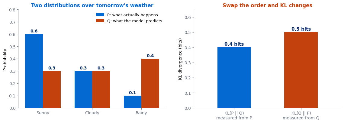
Here are the two distributions in the figure:
| Weather | P (reality) | Q (model) | P · log2(P/Q) |
|---|---|---|---|
| Sunny | 0.6 | 0.3 | 0.6 × log2(2) = 0.6 |
| Cloudy | 0.3 | 0.3 | 0.3 × log2(1) = 0 |
| Rainy | 0.1 | 0.4 | 0.1 × log2(0.25) = −0.2 |
| Total | 1.0 | 1.0 | KL(P || Q) = 0.4 bits |
Sunny days are twice as common as the model thinks, so they add 0.6 bits. Cloudy days are predicted perfectly, so they add nothing. Rainy days are over-predicted, which gives a negative term, but it is small because rain only happens 10% of the time. The total, 0.4 bits, is the average extra surprise per day from using the model instead of the truth.
Individual terms can be negative, but the total never is. KL divergence is always zero or positive, and it is exactly zero only when P and Q are identical.
Why KL divergence is not symmetric
Now swap the roles and compute KL(Q || P), weighting by Q instead:
🧪 The reverse direction
0.3 × log2(0.3 / 0.6) = 0.3 × −1 = −0.3Cloudy:
0.3 × log2(0.3 / 0.3) = 0Rainy:
0.4 × log2(0.4 / 0.1) = 0.4 × 2 = 0.8KL(Q || P) = 0.5 bits, not 0.4.
The difference comes from the weights. In this direction, rain carries 40% of the weight, and
P says rain is rare, so every rainy day is a big surprise. Going the other way, rain carried only 10% of the weight and barely mattered.This is why it is called a divergence and not a distance. A distance between A and B should equal the distance between B and A; KL does not. The order you write matters, so always read KL(P || Q) as “the cost of using Q when the truth is P“.
The asymmetry has practical consequences. Minimising KL(P || Q) punishes Q heavily for giving low probability to anything P considers likely, so Q spreads out to cover everything. Minimising KL(Q || P) punishes Q for putting weight where P has little, so Q tends to lock onto one peak and ignore the rest. These are often called mean-seeking and mode-seeking behaviour.
Cross-entropy = entropy + KL divergence
KL divergence has a close relative you have probably already used. The entropy of P, H(P) = −Σ P log P, is the unavoidable surprise built into the weather itself. The cross-entropy, H(P, Q) = −Σ P log Q, is the surprise you actually experience when you predict with Q. The gap between them is exactly the KL divergence:
H(P, Q) = H(P) + KL(P || Q)
Check it with the weather numbers. The entropy of P is −(0.6 log2 0.6 + 0.3 log2 0.3 + 0.1 log2 0.1) = 1.295 bits. The cross-entropy is −(0.6 log2 0.3 + 0.3 log2 0.3 + 0.1 log2 0.4) = 1.695 bits. And 1.295 + 0.4 = 1.695. It works.
The same holds for binary cross-entropy, which is just the two-outcome case, and it is part of why cross-entropy is the default loss function for classification.
Where KL divergence is used
Variational autoencoders (VAEs). A VAE compresses each input into a small cloud of possible codes, described by a mean and a spread. Its loss has two parts: how well it reconstructs the input, and a KL term that keeps each code distribution close to a standard normal. The KL term keeps the latent space smooth and tidy, which is what lets you sample new images from it. For two normal distributions the KL has a neat closed form, so no sampling is needed to compute it.
Knowledge distillation. A small “student” network learns to copy a large “teacher”. Instead of training only on hard labels, the student minimises the KL divergence between its softmax outputs and the teacher’s, usually softened with a temperature so that the teacher’s second and third choices carry information. The student learns that a picture of a husky is “mostly dog, slightly wolf”, which hard labels never tell it.
RLHF penalties. When a large language model is tuned with reinforcement learning from human feedback, it is rewarded for answers people prefer. Left alone, it can drift into strange text that games the reward model. A penalty proportional to the KL divergence between the tuned model and the original keeps it close to the language it already knew. A larger penalty weight means a more conservative update. It is a key reason fine-tuned models stay fluent.
You will also meet KL divergence in t-SNE visualisations, in monitoring whether production data has drifted from training data, and in Bayesian methods that approximate a complicated distribution with a simpler one.
⚠️ Pitfalls when computing it
- Zeros blow it up. If
Qgives probability 0 to an outcome thatPsays can happen,KL(P || Q)is infinite. Smooth or clip probabilities before computing it. - PyTorch’s argument order is unusual.
F.kl_div(input, target)expectsinputas log-probabilities of the model andtargetas probabilities, and computesKL(target || model). Passing plain probabilities asinputgives wrong numbers without any error. - Use
reduction="batchmean"in PyTorch. The default averages over every element, not every example, so the value does not match the mathematical definition. - Bits versus nats.
scipy.stats.entropy(p, q)returns KL divergence in nats unless you passbase=2. The weather example gives 0.277 nats, the same as 0.4 bits.
The calculation relies on nothing more than the logarithm rule log(a/b) = log a − log b, which is exactly how the cross-entropy relation above falls out of the formula.
🔑 Key Takeaways
- KL divergence,
Σ P log(P/Q), is the extra surprise from predicting withQwhen the truth isP. - It is always zero or positive, and zero only when the two distributions match.
- It is not symmetric: in the weather example,
KL(P || Q) = 0.4bits butKL(Q || P) = 0.5bits. - Cross-entropy equals entropy plus KL, so minimising cross-entropy loss minimises KL divergence.
- VAEs, knowledge distillation and RLHF penalties all rely on it to keep one distribution close to another.
Further reading
The Wikipedia article on Kullback–Leibler divergence covers its properties and the closed form for normal distributions, and the PyTorch KLDivLoss documentation spells out the argument order and reduction settings described above.
Where to go next
- Cross-entropy loss — the training loss KL divergence hides inside
- The softmax function — how models turn scores into the distributions KL compares
- Fine-tuning, prompting and RAG — where RLHF fits in adapting a model
- Start Here — the full learning path