Computers need numbers, and the obvious way to turn words into numbers, giving each word an ID or a one-hot column, says nothing about meaning. To such a system “cat” is exactly as different from “kitten” as it is from “carburettor”. Word2vec, published by Tomas Mikolov and colleagues at Google in 2013, was the method that made learned word vectors fast, cheap and famous, and it is the direct ancestor of the embeddings inside every modern language model.
The company a word keeps
The idea behind word2vec is much older than the algorithm. In 1957 the linguist J. R. Firth wrote: “You shall know a word by the company it keeps.” This is the distributional hypothesis: words that appear in similar contexts tend to have similar meanings.
Think about the sentences “I poured the ___ into a mug” and “the ___ had gone cold”. Coffee fits, tea fits, cocoa fits; granite does not. You never need a dictionary to know that coffee and tea are related. You only need to notice that they turn up surrounded by the same words. Word2vec turns that observation into a training signal.
The training task: a fake problem with a useful side effect
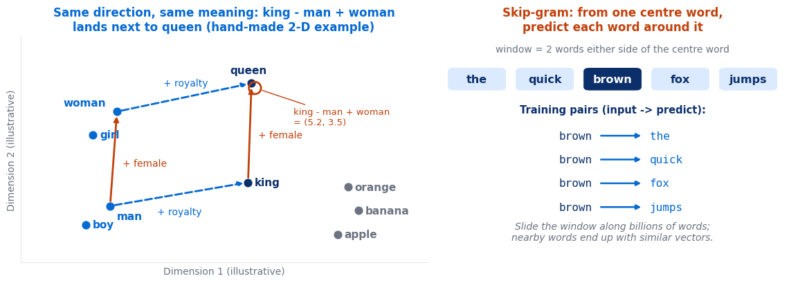
Word2vec sets up a prediction task that nobody actually cares about, then keeps the weights and throws the predictor away. Slide a window along a large body of text. Inside each window there is a centre word and its neighbours, say two on either side. The right-hand side of the figure shows the window around “brown” in “the quick brown fox jumps”, which produces four training pairs: (brown, the), (brown, quick), (brown, fox) and (brown, jumps).
The network itself is tiny: a lookup table, called the embedding matrix, with one row of, say, 300 numbers per word, followed by an output layer. Given a word, you look up its row and use it to score every possible neighbour. Training nudges the rows so real neighbours score highly. Because “coffee” and “tea” have to predict the same neighbours (“mug”, “cup”, “drink”, “hot”), the easiest way for the network to do well is to give them similar rows. Those rows are the word vectors.
Skip-gram vs CBOW
Word2vec comes in two flavours, which are mirror images of each other.
- Skip-gram uses the centre word to predict each surrounding word, as in the figure. It produces more training pairs per sentence and does better on rare words, so it is the usual choice for smaller datasets.
- CBOW (continuous bag of words) does the reverse: it averages the vectors of the surrounding words and uses that to predict the centre word, like a fill-in-the-blank exercise. It trains several times faster and does slightly better on frequent words.
Both learn vectors of similar quality. In practice the choice matters less than the amount of text and the window size: small windows of 2 to 5 tend to capture grammatical similarity (running, walking, jumping), while larger windows capture topic (running, marathon, trainers).
🧪 Worked example: how big is the model, and why negative sampling?
Predicting a neighbour with a full softmax means scoring all 50,000 words for every single training pair, which is far too slow over billions of pairs.
Negative sampling replaces that with a yes-or-no question. For the real pair (brown, fox), also draw 5 random words, say (brown, tax), (brown, seven) and so on, and train the model to say “real” for the first and “fake” for the rest. That is 6 scores per pair instead of 50,000, roughly 8,000 times less work.
King − man + woman ≈ queen
The result that made word2vec famous is that directions in the vector space carry meaning. The difference between “man” and “woman” is roughly the same vector as the difference between “king” and “queen”, and between “uncle” and “aunt”. The same happens for other relations: countries and capitals, verbs and their past tenses, adjectives and their comparatives.
So you can do arithmetic with meaning. Using the illustrative coordinates in the figure: king is (5.0, 1.5), man is (1.0, 1.0) and woman is (1.2, 3.0). Subtract man from king and add woman: (5.0 − 1.0 + 1.2, 1.5 − 1.0 + 3.0) = (5.2, 3.5). The nearest word is queen at (5.1, 3.6), just 0.14 away. Real word2vec vectors have 300 dimensions, and “nearest” is measured with cosine similarity, but the arithmetic is exactly this.
Nobody told the model about gender or royalty. Those directions emerged only because words like “he”, “his”, “crown” and “throne” appear in consistent patterns around them.
⚠️ The limits of word2vec
- One vector per word, so no context. “Bank” gets a single vector that blends the river bank and the bank that lends money. “I sat by the bank” and “I paid the bank” look identical to it.
- Unknown words get nothing. A word that never appeared in training has no vector at all. FastText, a later variant, fixes this by building vectors from pieces of words.
- Opposites look similar. “Hot” and “cold” appear in the same company (“the water was ___”), so they sit close together even though they mean the reverse.
- Analogies are cherry-picked. The famous examples work, but many do not, and the standard test quietly excludes the input words, because otherwise the nearest answer to king − man + woman is often “king” itself.
- It learns the text’s biases. Trained on news articles, analogies such as man is to programmer as woman is to homemaker appear. The vectors mirror the data, prejudices included.
How word2vec relates to modern embeddings
The first limit is the one that mattered most, and fixing it is the story of modern NLP. Contextual models give a word a different vector each time it appears, depending on the sentence around it. In a transformer, “bank” in “river bank” and “bank loan” starts from the same vector, and then layers of attention mix in information from the neighbouring words until the two vectors point in clearly different directions.
That starting vector is a direct descendant of word2vec. The first layer of every large language model is still a lookup table with one learned row per token, trained on the same principle of predicting words from their company. The differences are that the table is trained together with the rest of the model, the tokens are word pieces rather than whole words, and the context is thousands of tokens rather than a window of five.
🔑 Key Takeaways
- Word2vec learns word vectors from the distributional hypothesis: a word is known by the company it keeps.
- Skip-gram predicts neighbours from the centre word; CBOW predicts the centre word from its neighbours.
- Negative sampling turns an expensive 50,000-way prediction into a handful of yes-or-no questions.
- Directions carry meaning, so king − man + woman lands near queen, though many analogies fail.
- One vector per word ignores context, which is exactly what transformer embeddings fixed.
Further reading
The original paper, Efficient Estimation of Word Representations in Vector Space by Mikolov and colleagues, introduced skip-gram and CBOW. To train your own vectors, the gensim Word2Vec documentation covers every parameter mentioned here.
Where to go next
- Embeddings explained — how machines measure meaning, and how modern embeddings build on word2vec
- Tokenisation explained — why modern models embed word pieces rather than words
- Attention explained — how context gets mixed into each vector
- Start Here — the full learning path