Entropy in machine learning sounds like physics, but the idea is simple: how unpredictable is this? A label column that is half spam and half not-spam is very unpredictable. A column that is 99% not-spam is barely unpredictable at all. Entropy puts a number on that difference, and once you have the number, two of the most common tools in ML fall out of it almost for free.
Entropy as surprise
Start with a single outcome. If something had a 50% chance and it happened, you are mildly surprised. If it had a 1% chance, you are very surprised. If it was certain, you are not surprised at all.
Information theory measures the surprise of an outcome with probability p as -log2(p). The logarithm is what makes this behave sensibly:
- An outcome with
p = 1gives-log2(1) = 0. No surprise. - An outcome with
p = 0.5gives-log2(0.5) = 1. One unit of surprise. - An outcome with
p = 0.1gives-log2(0.1) = 3.32. Rare events are much more surprising.
Entropy is simply the average surprise, weighting each outcome by how often it happens:
H = -Σ p(x) · log2 p(x)
In words: for every possible outcome, multiply its probability by its surprise, then add the results up.
Three coins, worked out
🧪 Worked example: fair, biased and certain
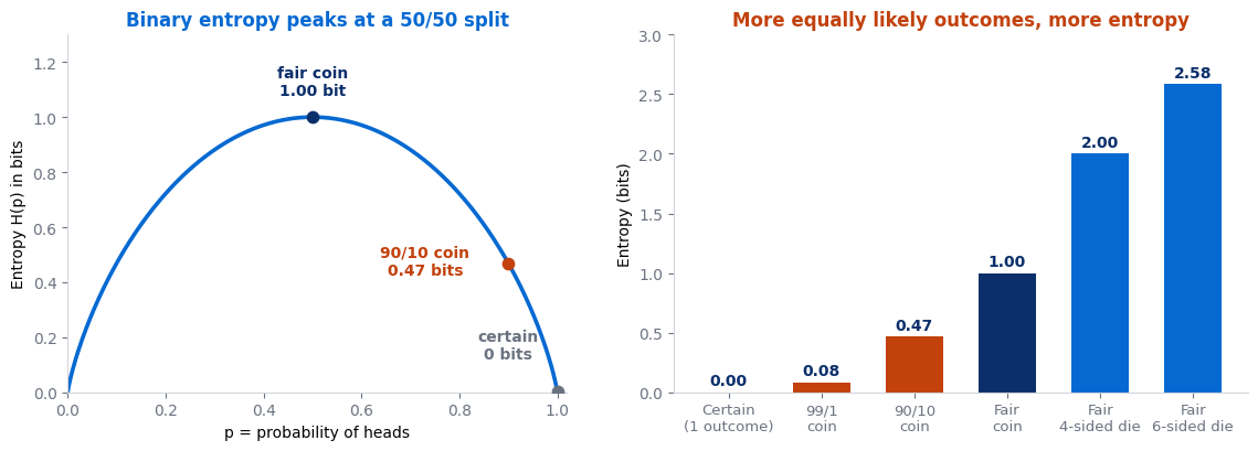
-log2(0.5) = 1 bit. Average: 0.5 × 1 + 0.5 × 1 = 1.00 bit.Biased coin (90% heads, 10% tails). Heads has surprise
-log2(0.9) = 0.152 bits; tails has -log2(0.1) = 3.32 bits. Average: 0.9 × 0.152 + 0.1 × 3.32 = 0.137 + 0.332 = 0.47 bits. Tails is very surprising, but it rarely happens, so the average is low.Certain outcome (100% heads).
1 × -log2(1) = 0 bits. You learn nothing by watching it.The left panel of the figure traces this for every possible coin. It is a hill: zero at both ends, where the coin always lands the same way, and a peak of exactly 1 bit in the middle, where you genuinely cannot guess. The right panel adds more outcomes. A fair four-sided die has 2 bits of entropy and a fair six-sided die has 2.58 bits. In general, k equally likely outcomes give log2(k) bits, the maximum possible for k outcomes.
What the units mean
When you use log2, entropy is measured in bits. One bit is the uncertainty of one fair yes/no question. That gives a handy interpretation: 2 bits for the four-sided die means you need, on average, two well-chosen yes/no questions to identify the result (“Is it 1 or 2?”, then “Is it 1?”).
Most ML libraries use the natural log instead, which gives nats. The ideas are identical; only the scale changes. One nat is about 1.44 bits, so a fair coin has 1 bit or 0.693 nats. When a training log reports a loss of 0.69 on a balanced binary problem, that is the model being exactly as uncertain as a fair coin.
ln(10) = 2.30. If your first epoch starts far above these, something is wrong with your initialisation or labels.Where entropy shows up in machine learning
1. Decision tree splits and information gain
A decision tree grows by repeatedly asking which question best separates the classes. Entropy gives a precise answer. Measure the entropy of the labels before the split, measure the weighted entropy of the two groups after it, and the drop is called information gain. The tree picks the split with the largest gain.
Take 10 emails: 5 spam and 5 not spam. The entropy of the labels is 1 bit, as uncertain as it gets.
- Split on “contains the word free“. One side gets 5 emails (4 spam, 1 not); the other gets 5 (1 spam, 4 not). Each side has entropy
H(0.8, 0.2) = 0.722bits. Weighted average:0.5 × 0.722 + 0.5 × 0.722 = 0.722. Information gain:1 − 0.722 = 0.278bits. - Split on “sent on a weekday”. One side gets 6 emails (3 spam, 3 not), the other 4 (2 spam, 2 not). Both sides are still 50/50, so both have entropy 1 bit. Information gain: 0.
The tree chooses “contains free” because it removes more uncertainty. The same calculation, repeated at every node, builds the whole tree, and by extension the random forests and gradient boosting models built from many trees.
In scikit-learn you switch this on with DecisionTreeClassifier(criterion="entropy"). The default, Gini impurity, is a cheaper cousin that almost always picks the same splits.
2. Cross-entropy loss
Entropy measures the surprise when you know the true probabilities. Cross-entropy measures the surprise when reality follows one distribution but you are predicting with another:
H(p, q) = -Σ p(x) · log q(x)
Here p is the truth and q is the model’s prediction. For a classification label, p puts all its weight on the correct class, so the sum collapses to one term: -log q(correct class). If the model gives the correct class 0.7, the loss is -ln(0.7) = 0.357 nats. If it gives it only 0.1, the loss is -ln(0.1) = 2.30 nats. The model is penalised by exactly how surprised it was by the right answer.
That is why cross-entropy loss is the standard loss function for classifiers, usually applied to the output of a softmax. For yes/no problems the two-class version is binary cross-entropy. Cross-entropy can never be lower than the true entropy of the labels; the gap between the two is a separate quantity called KL divergence, which measures how far the model’s distribution sits from the truth.
3. Other places you will meet it
- Language models are trained with cross-entropy on the next token, and their “perplexity” score is just
2^H(ore^H): the number of equally likely tokens the model is effectively choosing between. - Active learning picks the unlabelled examples where the model’s predicted distribution has the highest entropy, because those are the ones it is least sure about.
- Feature selection uses mutual information, the information gain idea applied to a single feature against the target.
⚠️ Three common slips
log(0)is minus infinity. By convention an outcome with probability 0 contributes 0 to entropy. In cross-entropy, a model that predicts exactly 0 for the true class gets infinite loss, which is why libraries clip probabilities to a tiny minimum.- Mixing bits and nats. A paper reporting 1.0 and a library reporting 0.693 may describe the same thing. Check the log base before comparing numbers.
- High entropy is not “bad”. It describes the data, not the model. A balanced dataset has high label entropy by design; what matters is how much a model or split reduces it.
Entropy in a few lines of Python
You rarely need to code it yourself, but doing so once makes the formula stick:
import numpy as np; p = np.array([0.9, 0.1]); H = -(p * np.log2(p)).sum() gives 0.469.
For real work, scipy.stats.entropy(p, base=2) does the same and handles zeros for you. If you want the wider picture of probability distributions this builds on, the statistics for machine learning guide covers the groundwork.
🔑 Key Takeaways
- Entropy is the average surprise,
H = -Σ p log p: high when outcomes are equally likely, zero when one is certain. - A fair coin has 1 bit, a 90/10 coin 0.47 bits, and
kequally likely outcomeslog2(k)bits. - Bits use
log2, nats use the natural log; 1 bit is about 0.693 nats. - Decision trees choose the split with the highest information gain, the biggest drop in entropy.
- Cross-entropy loss is the surprise the model feels at the correct answer,
-log q(correct class).
Further reading
The Wikipedia article on entropy in information theory traces the idea back to Claude Shannon’s 1948 paper, and scikit-learn’s decision tree classification criteria set out the entropy and Gini formulas exactly as the library computes them.
Where to go next
- Decision trees explained — see information gain building a real tree
- Cross-entropy loss — entropy turned into a training objective
- Logarithms explained — the maths behind every formula on this page
- Start Here — the full learning path