If you only ever tune one setting, make it the learning rate. It decides whether training takes minutes or days, and whether it works at all. The same model on the same data can go from useless to excellent by changing this one number by a factor of ten.
What the learning rate does
Training by gradient descent repeats one update: w = w - lr * gradient. The gradient says which way is downhill on the loss and how steep it is. The learning rate, lr, says how far to move in that direction. It is a hyperparameter: you choose it, the model does not learn it.
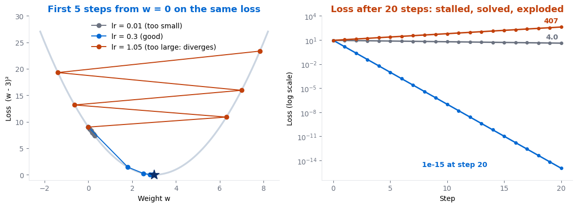
Three runs on the same loss
The figure uses the simplest possible loss, L(w) = (w - 3)², whose minimum is at w = 3. Its gradient is 2(w - 3). Every run starts at w = 0, where the loss is 9. Only the learning rate changes.
🧪 First step, three ways
lr = 0.01: w moves to 0 + 0.06 = 0.06. Each step closes just 2% of the gap to 3. After 20 steps w is only 1.0 and the loss is still 4.0.
lr = 0.3: w moves to 0 + 1.8 = 1.8. Each step closes 60% of the gap. After 20 steps the loss is effectively zero.
lr = 1.05: w moves to 0 + 6.3 = 6.3. It has jumped right over the minimum and landed higher up the other side (loss 10.9). The next step overshoots again, further each time, and after 20 steps the loss is 407.
For this loss the gap to the minimum is multiplied by
1 - 2 × lr on every step. Below lr = 0.5 you creep; at exactly 0.5 you land on the minimum in one step; between 0.5 and 1 you overshoot but still settle; above 1 you diverge.Too small, too large, and divergence
Too small is the quiet failure. Nothing breaks, the loss falls steadily, and it looks as if the model is learning. It is just learning so slowly that you run out of time or patience, and you may wrongly conclude that the model or the features are weak.
Slightly too large shows up as a loss that falls fast and then bounces around a floor instead of settling. The steps are too big to get into the bottom of the valley.
Far too large is divergence. Each step overshoots by more than the last, the loss climbs instead of falls, and within a few hundred steps it becomes inf or NaN. If your training log suddenly prints NaN, a too-high learning rate is the first suspect.
Why is there a hard ceiling? The safe step size depends on how sharply the loss curves. A steep, narrow valley needs small steps; a wide, gentle one tolerates big ones. Our parabola has a curvature of 2, which puts the cliff edge at lr = 1. Real neural networks have millions of directions with different curvatures, and the sharpest one sets the limit for all of them. That is also why scaling your features helps: it makes the valley rounder, so one learning rate suits every direction.
⚠️ Reading a training curve
- Loss falls in a slow straight line: learning rate too small. Try 3 to 10 times larger.
- Loss drops fast, then jitters at a plateau: slightly too large. Add decay, or halve it.
- Loss rises, or becomes NaN: far too large. Divide by 10.
- Changing batch size? The best learning rate usually changes with it. Larger batches give cleaner gradients and tolerate larger steps.
How to pick one: the learning-rate range test
Guessing and retraining is slow. The range test, popularised by Leslie Smith, finds a good value in a single short run:
- Start with a tiny learning rate, such as 0.0000001.
- After every mini-batch, multiply it by a constant so that it reaches about 10 after 100 to 300 batches.
- Record the training loss at each learning rate and plot loss against learning rate on a log scale.
- The loss will be flat at first, then fall steeply, then shoot up. Pick a value where the loss is falling fastest, typically about ten times lower than the point where it bottoms out.
If the loss is lowest at 0.1 and explodes at 0.3, a learning rate of about 0.01 is a safe start. The whole test costs a fraction of one epoch, far less than a grid search. Libraries such as fastai have it built in as lr_find().
Schedules and decay
The best learning rate early in training is not the best one late in training. Early on you are far from the minimum and want big strides. Near the end, big strides make you bounce around the bottom. A schedule changes the learning rate as training runs.
| Schedule | What it does |
|---|---|
| Step decay | Multiply by 0.1 at fixed epochs, for example 0.1 then 0.01 then 0.001 at epochs 30 and 60 |
| Exponential decay | Multiply by a factor such as 0.95 every epoch, a smooth version of step decay |
| Cosine annealing | A popular default. Glides from the starting rate down to near zero along a half cosine curve |
| Warm-up | Ramps up from near zero over the first few hundred steps, then hands over to decay; standard for transformers |
| Reduce on plateau | Halves the rate whenever validation loss stops improving for a set number of epochs |
Decay also acts as a mild guard against overfitting: the final small steps settle the weights instead of letting them keep jumping between noisy mini-batches.
Adam and adaptive learning rates
Optimisers such as Adam, RMSprop and Adagrad give every weight its own effective step size. Adam tracks a running average of each weight’s gradients and of their squares, then divides the step by the square root of the second. Weights with large, consistent gradients get tempered steps; weights with small, rare gradients get boosted ones.
This makes Adam much less fussy, and its default of 0.001 works surprisingly often. But adaptive does not mean automatic. Adam still has a global learning rate that scales everything, it can still diverge if that is too high, and it still benefits from warm-up and decay. Treat 0.001 as a starting point for your range test, not a final answer.
🔑 Key Takeaways
- The learning rate scales every update:
w = w - lr * gradient. - Too small crawls, slightly too large jitters, far too large diverges to NaN.
- On
(w - 3)², lr = 0.01 leaves the loss at 4.0 after 20 steps, lr = 0.3 solves it, and lr = 1.05 blows it up to 407. - A learning-rate range test finds a good value in one short run; search on a log scale.
- Use a schedule to shrink the rate over time, and treat Adam’s 0.001 as a starting point, not a guarantee.
Further reading
Leslie Smith’s paper Cyclical Learning Rates for Training Neural Networks introduced the range test, and the PyTorch optimiser documentation lists every built-in schedule with its parameters.
Where to go next
- Hyperparameter tuning — how to search the other settings once the learning rate is right
- Backpropagation — where the gradients that the learning rate scales come from
- The vanishing gradient problem — when no learning rate can fix slow training
- Start Here — the full learning path