Backpropagation has a reputation for being hard. It is not. It is one rule from calculus — the chain rule — applied over and over, with the results stored so nothing is computed twice.
This post assumes you have read how a neural network layer works.
The problem backpropagation solves
Your network makes a prediction. It is wrong by some amount. Somewhere among thousands of weights, some pushed the prediction too high and some too low.
The naive approach would be to nudge each weight individually, re-run the network, and see what happens. For a million weights, that is a million forward passes per training step — completely impractical. Backpropagation gets every gradient in one backward pass.
Forward pass, then backward pass
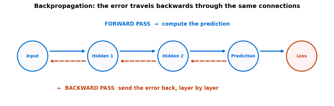
Forward: push the input through each layer, computing a = f(Wx + b) as you go, and keep every intermediate value — you will need them shortly. At the end, compare the prediction with the truth using a loss function.
Backward: start at the loss and walk back. At each layer, work out how sensitive the loss is to that layer’s output, then use it to get two things: the gradients for this layer’s weights, and the sensitivity to pass to the layer before.
The chain rule, which is all backpropagation is
If a change in w changes z, and a change in z changes the loss L, then the effect of w on L is the two effects multiplied:
$$\frac{\partial L}{\partial w} = \frac{\partial L}{\partial z} \times \frac{\partial z}{\partial w}$$
🧪 The intuition: a chain of gears
A neural network is a chain of gears from every weight to the loss. Backpropagation multiplies the ratios along each chain. It works backwards rather than forwards purely because that way the shared parts of the chain get computed once instead of thousands of times.
A worked backpropagation example
The smallest useful case: one input, one weight, no activation, squared error.
🧪 One weight, worked end to end
Forward: z = 2 × 3 = 6. Loss = (6 − 10)² = 16.
Backward, step 1 — how does the loss change with the prediction?
∂L/∂z = 2(z − y) = 2(6 − 10) = −8
Backward, step 2 — how does the prediction change with the weight?
∂z/∂w = x = 3
Multiply along the chain:
∂L/∂w = −8 × 3 = −24
Read it: the gradient is negative, so increasing w decreases the loss. Gradient descent therefore steps w up. With a learning rate of 0.01: w ← 2 − (0.01 × −24) = 2.24.
Check: new prediction = 2.24 × 3 = 6.72, new loss = (6.72 − 10)² = 10.76. Down from 16. It worked.
A real network does exactly this, for every weight, with one extra multiplication per layer it passes through. That is the entire algorithm.
Why deep networks get hard to train
Because the chain rule multiplies, the gradient for an early layer is a product of many terms. If those terms are each smaller than one, the product shrinks fast — after twenty layers, a gradient of 0.5 per layer has become 0.5²⁰, which is about 0.000001. The early layers barely move.
⚠️ This is the vanishing gradient problem
Three things worth knowing
🔑 Key Takeaways
- Backpropagation computes how much each weight contributed to the loss.
- It is the chain rule applied backwards, reusing shared results so nothing is recomputed.
- Forward pass makes the prediction and stores intermediates; backward pass assigns blame.
- Multiplying many small derivatives is what causes vanishing gradients in deep networks.
- Backpropagation finds the direction; gradient descent takes the step.
Further reading
3Blue1Brown’s visual walkthrough of backpropagation is worth twenty minutes of anyone’s time, and PyTorch’s autograd tutorial shows the same computation happening automatically in code.
Where to go next
- The vanishing gradient problem — what goes wrong, and the fixes
- The chain rule — the calculus underneath
- Activation functions — and why their derivatives matter so much
- Start Here — the full learning path