Every “because you watched”, “customers also bought” and auto-generated playlist is a recommender system at work. The problem they solve is easy to state: you know a few things each user liked, so guess what else they will like. The catch is that you know very little about each user.
The user-item matrix, and why it is mostly empty
Put users in rows and items in columns, and write each known rating in its cell. That grid is the user-item matrix, and every recommender is trying to fill in its blanks. Below is a toy version: five people, six films, ratings from 1 to 5.
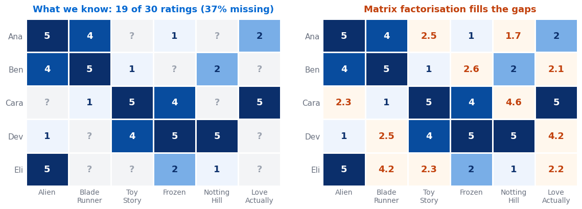
Here 37% of the cells are missing. That is wildly optimistic. In the Netflix Prize dataset, 480,189 users rated 17,770 films about 100 million times, which fills roughly 1.2% of the matrix. More than 98% of the cells were blank. This sparsity is the central fact of recommender systems: you can’t treat the blanks as zeros, because a blank means “not seen”, not “hated”. Filling the gaps is a kind of missing-data problem, and the gaps are also exactly the items you want to recommend.
Content-based vs collaborative filtering
There are two basic ways to fill a blank.
Content-based filtering describes each item with features: genre, director, keywords, price, or an embedding of its text or image. It builds a profile of what each user liked, then recommends items whose features match. If Eli rated Alien 5, a content-based system suggests more sci-fi horror. It needs no other users, but it tends to recommend more of the same.
Collaborative filtering ignores item descriptions completely. It only looks at the pattern of ratings: people who agreed with you in the past will probably agree with you again. It can find links no feature list would capture, but it needs plenty of rating data.
| Content-based | Collaborative filtering | |
|---|---|---|
| Uses | Item features + one user’s history | Everyone’s ratings, no item features |
| New item | Fine, as soon as it has features | Invisible until people rate it |
| Surprise | Low, more of the same | Higher, can cross categories |
| In practice | Hybrids. Most production systems combine the two, often by feeding content features into a collaborative model. | |
A worked example: user-based collaborative filtering
The simplest collaborative method is a nearest-neighbours idea. Find the users most similar to Eli, then average their ratings for the film you want to predict, weighted by how similar they are. To measure similarity you compare the ratings two users share, and the usual tool is cosine similarity: the dot product of the two rating vectors divided by the product of their lengths.
🧪 Should we recommend Blade Runner to Eli?
Eli vs Ana (Alien, Frozen): Eli (5, 2), Ana (5, 1). Dot product 25 + 2 = 27. Lengths √29 = 5.39 and √26 = 5.10. Cosine = 27 / 27.46 = 0.983.
Eli vs Ben (Alien, Notting Hill): (5, 1) vs (4, 2). Dot 22, lengths 5.10 and 4.47. Cosine = 0.965.
Eli vs Dev (Alien, Frozen, Notting Hill): (5, 2, 1) vs (1, 5, 5). Dot 20, lengths 5.48 and 7.14. Cosine = 0.511.
Ana gave Blade Runner 4 and Ben gave it 5. The weighted average is (0.983 × 4 + 0.965 × 5) / (0.983 + 0.965) = 8.757 / 1.948 = 4.50. Recommend it. The matrix factorisation in the figure reaches a similar answer, 4.2, by a different route.
⚠️ Two traps hiding in that calculation
- Tiny overlaps give fake certainty. Cara shares only one film with Eli (Frozen), so their cosine is a perfect 1.000. Let her vote on Blade Runner, which she rated 1, and the prediction falls from 4.50 to 3.31. Require a minimum overlap, or shrink similarities built on few items.
- Raw ratings are all positive, so everyone looks similar. Dev’s taste is the opposite of Eli’s, yet their cosine is still 0.51. Subtract each user’s average rating first (so a 2 from a generous rater counts as negative). This mean-centred version is essentially Pearson correlation, and it is the usual fix.
Matrix factorisation in plain words
Neighbour methods get slow and noisy once you have millions of users. The approach at the heart of the Netflix Prize winners, and still behind many systems, is matrix factorisation.
The idea: suppose each film can be summarised by a handful of hidden scores, say “how sci-fi” and “how romantic”, and each user by how much they care about each of those. A predicted rating is then the dot product of the user’s taste scores and the film’s scores, plus the overall average. Nobody labels these factors. The model learns them by adjusting both sets of scores until their dot products match the ratings you do have, ignoring the blanks.
In the figure, two factors per user and per film (22 numbers in total) reproduce the 19 known ratings with a root-mean-square error of 0.42 stars, and the orange cells are what those same factors imply for the blanks. It is closely related to singular value decomposition, which breaks a full matrix into the same kind of low-rank pieces. Classic SVD needs every cell filled, though, so recommenders fit the factors to the observed cells only, usually by alternating least squares or gradient descent, with L2 regularisation to stop the factors memorising the few ratings a user has.
Cold start
Collaborative filtering has nothing to say about a user or item with no history. A brand-new film has an empty column, so no one’s taste can reach it. A new user has an empty row, so there is no one to compare them with. This is the cold start problem, and every real system needs a plan for it:
- New users: ask for a few favourites at sign-up, start with popular items, or use context such as location, device and the page they arrived from.
- New items: fall back on content features (genre, text, image embeddings) until ratings arrive. This is the main reason hybrids exist.
- Deliberate exploration: show new items to a small slice of users so they can collect their first ratings.
Popularity bias
Popular items have more ratings, so the model is more confident about them and ranks them higher. They are then shown more and collect even more ratings. Left alone, a recommender turns into a bestseller list, and the long tail of niche items, often the most useful suggestions, never gets a chance. Watch for it by measuring coverage (what share of your catalogue ever gets recommended) alongside accuracy. Common countermeasures are down-weighting popular items, re-ranking for diversity, and the exploration mentioned above.
Implicit vs explicit feedback
Explicit feedback is a user telling you directly what they think: star ratings, thumbs up or down. It is clear, but scarce, because most people never rate anything.
Implicit feedback is inferred from behaviour: clicks, plays, watch time, purchases, add-to-basket. It is plentiful and it is what most modern systems train on, but it is harder to read. A play might be a mis-click. An unwatched film might be disliked or simply undiscovered, so implicit data has no true negatives. The standard approach treats interactions as positives with a confidence that grows with repetition (ten plays count more than one), and samples non-interacted items as weak negatives. The goal changes too: you stop predicting a star rating and start ranking items by how likely the user is to engage. Careful feature engineering on behaviour signals, such as the share of an episode actually watched, often matters more than the algorithm.
🔑 Key Takeaways
- Recommender systems fill in a user-item matrix that is usually more than 98% empty, and a blank means “unseen”, not “disliked”.
- Content-based filtering matches item features; collaborative filtering borrows the ratings of similar users. Real systems mix both.
- User similarity by cosine needs a minimum overlap and mean-centred ratings, or it gives confident nonsense.
- Matrix factorisation learns a few hidden taste scores per user and item, and their dot product predicts the blanks.
- Plan for cold start and popularity bias from day one, and expect to train on implicit feedback rather than star ratings.
Further reading
Wikipedia’s article on collaborative filtering covers the neighbour and model-based families in more depth, and the Surprise library lets you try user-based filtering and SVD-style factorisation on real rating data in a few lines of Python.
Where to go next
- Cosine similarity calculator: check the worked example yourself
- Singular value decomposition: the linear algebra behind matrix factorisation
- Embeddings: the learned taste vectors, in a more general form
- Start Here: the full learning path