A random forest grows many trees independently and averages them. Gradient boosting grows them in sequence, and that one change makes it both more accurate and more dangerous.
How gradient boosting works
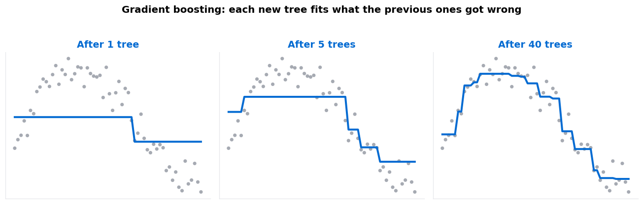
The loop is short:
- Start by predicting the average for everything.
- Compute the residuals — how wrong you are on each row.
- Fit a small tree to predict those residuals.
- Add a fraction of that tree’s predictions to your running total.
- Repeat, hundreds of times.
Where the “gradient” comes in
Fitting the residuals is not an arbitrary choice. For squared-error loss, the residual is the negative gradient of the loss function with respect to the prediction.
So each tree is a step downhill on the loss surface — the same gradient descent idea used everywhere else, except the step is taken by adding a tree rather than by nudging a weight. That framing is what lets boosting optimise any differentiable loss, not just squared error.
The two settings that matter
🧪 Learning rate and tree count trade off
Why deliberately slow it down? Because small, cautious steps generalise better than a few large ones — the model is less likely to leap onto a quirk of the training data.
The consequence is a direct trade: halve the learning rate and you need roughly twice as many trees. A low rate with many trees usually beats a high rate with few, at the cost of training time.
Sensible starting point: learning rate 0.05–0.1, then use early stopping to decide the tree count for you.
It can overfit — unlike a random forest
⚠️ More trees is not always better here
The fix is early stopping: watch performance on a validation set and stop when it stops improving. Every serious boosting library supports this, and you should always use it. See overfitting and underfitting.
XGBoost, LightGBM and CatBoost
All three implement the same algorithm with different engineering. For a first project, any of them will do; CatBoost asks least of you if your data has many categorical columns.
Boosting versus a random forest
| Random forest | Gradient boosting | |
|---|---|---|
| Trees built | Independently, in parallel | Sequentially, each fixing the last |
| Tree depth | Deep | Shallow |
| More trees | Never hurts | Can overfit |
| Tuning | Forgiving | Rewards care |
| Typical accuracy | Very good | Usually best on table data |
A reasonable working habit: start with a random forest for a quick strong baseline, then move to boosting when you want the last few points and are willing to tune.
🔑 Key Takeaways
- Gradient boosting adds shallow trees in sequence, each fitting the previous errors.
- Residuals are the gradient of the loss — every tree is a step downhill.
- Lower learning rate needs more trees, and usually generalises better.
- Unlike a random forest, too many trees overfits — always use early stopping.
- Usually the strongest option on spreadsheet data; still beaten by neural networks on images and text.
Further reading
The XGBoost introduction to boosted trees derives the algorithm carefully, and scikit-learn’s histogram gradient boosting is a fast built-in implementation needing no extra install.
Where to go next
- Convolutional neural networks — the next post, and where boosting stops winning
- Random forests — the parallel alternative
- Hyperparameter tuning — boosting rewards it more than most
- Start Here — the full learning path