A model has two kinds of numbers. Parameters are learned during training. Hyperparameters are the ones you set beforehand — how deep the tree may go, how strong the regularisation is, how many neighbours vote. Hyperparameter tuning is finding good values for them.
What you are actually tuning
| Model | The hyperparameters that matter most |
|---|---|
| Decision tree | max_depth, min_samples_leaf |
| Random forest | n_estimators, max_depth, max_features |
| Gradient boosting | learning_rate, n_estimators, max_depth |
| k-NN | n_neighbors, the distance metric |
| Logistic regression | C (inverse regularisation), the penalty type |
Note that most of these control model complexity — which means hyperparameter tuning is, in practice, mostly about finding the right point between overfitting and underfitting.
Grid search versus random search
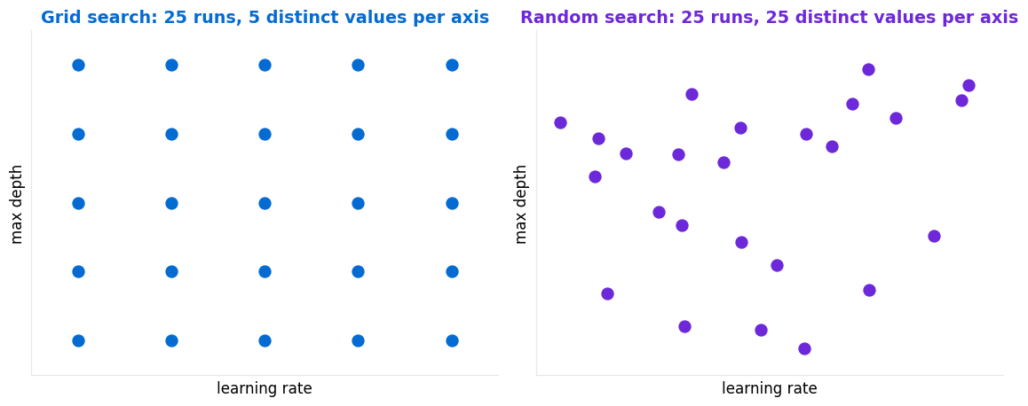
Grid search tries every combination in a grid you specify. Thorough, reproducible, and it explodes: 5 values across 4 hyperparameters is 625 combinations, and with 5-fold cross-validation that is 3,125 model fits.
Random search samples combinations at random from ranges you specify, for a fixed budget of runs.
Use grid search when you have two or three hyperparameters and a small set of sensible values. Use random search otherwise — it is the better default.
Search ranges that make sense
Some hyperparameters should be sampled on a log scale, not a linear one. The interesting difference between learning rates of 0.001 and 0.01 is far larger than between 0.10 and 0.11, so sampling uniformly from 0 to 1 wastes almost every run.
🧪 Sensible starting ranges
Linear scale: max_depth 3 → 20 · min_samples_leaf 1 → 50 · n_neighbors 1 → 30
And a rule worth remembering: if your best value sits at the edge of your range, the range was too narrow. Extend it and search again.
The mistake that makes tuning meaningless
⚠️ Never tune against your test set
Correct approach: hold out a test set at the very start and do not touch it. Tune using cross-validation on the remaining data. Evaluate the single winning configuration on the test set once, at the end.
The preprocessing rule applies here too — scaling and imputation must sit inside the pipeline being tuned, or every fold leaks.
Beyond random search
Bayesian optimisation uses the results so far to decide what to try next, concentrating on promising regions. Optuna is the usual tool. It is meaningfully more efficient when each training run is expensive; for a model that fits in seconds, random search with more runs is simpler and just as good.
Successive halving starts many configurations on a small slice of the data, discards the worst, and gives survivors more resources. Available in scikit-learn as HalvingRandomSearchCV.
How much does tuning actually buy you?
Less than beginners expect. Typical gains are one to three percentage points. Better features or more data will usually beat any amount of tuning, and a well-chosen model with default settings is often within a couple of points of a heavily tuned one.
🔑 Key Takeaways
- Hyperparameters are set before training; parameters are learned during it.
- Random search beats grid search for the same budget, because it tries more distinct values of each setting.
- Sample learning rates and regularisation strengths on a log scale.
- A best value at the edge of your range means the range was too narrow.
- Tune with cross-validation; touch the test set once, at the very end.
Further reading
scikit-learn’s tuning guide documents GridSearchCV, RandomizedSearchCV and the halving variants, and Optuna is the standard tool if you move on to Bayesian optimisation.
Where to go next
- Imbalanced datasets — the next post in this sequence
- Cross-validation — the machinery tuning depends on
- Feature engineering — usually worth more than tuning
- Start Here — the full learning path