Big neural networks have enough capacity to memorise almost any training set, noise included. Dropout is one of the cheapest defences against that: one extra line of code, no new data, and often a large drop in validation loss. It is also a little strange the first time you meet it, because it works by deliberately breaking the network while it learns.
What dropout actually does
During training, at every step and for every example, each neuron in a dropout layer is switched off with probability p. Switched off means its output is set to zero, so for that step it contributes nothing to the layers above and receives no gradient in backpropagation. On the next step a fresh random set is switched off.
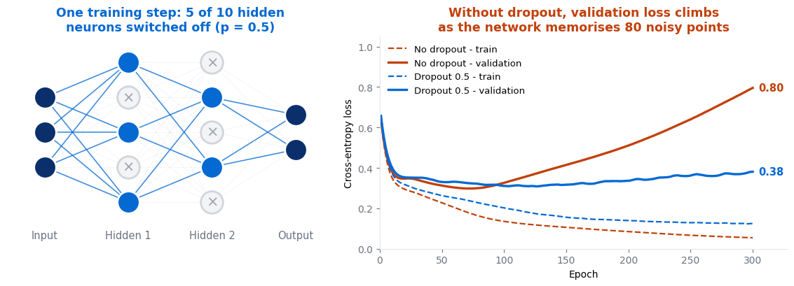
The right-hand panel comes from a real run. A network with two hidden layers of 256 neurons was trained for 300 epochs on just 80 noisy points and tested on 1,000 fresh ones. Without dropout, training loss falls to 0.05 while validation loss bottoms out around epoch 70 and then rises steadily to 0.80. That widening gap is textbook overfitting. With dropout at 0.5 the training loss stays higher, at 0.13, but validation loss ends at 0.38, less than half the other figure.
Notice what dropout did not do: the best validation loss is about 0.30 either way. Dropout rarely makes the ideal model better. What it does is make the network far less eager to wreck itself by memorising, so you have a much wider window in which it performs well.
Why randomly breaking a network helps
There are two good ways to think about it, and they are really the same idea seen from different angles.
No co-adaptation. Without dropout, neurons can form fragile partnerships: neuron A learns to fix up a quirk in neuron B’s output, which only exists because of one odd training example. Those partnerships are exactly what memorisation looks like inside a network. With dropout, A cannot count on B being present, so each neuron has to learn something that is useful on its own and alongside many different random sets of colleagues. The features that survive are more general.
A cheap ensemble. A layer of 256 neurons with dropout has 2256 possible “thinned” versions, one per pattern of switched-off neurons. Every training step trains one of them, and they all share the same weights. At test time, using the full network with rescaled weights is a good approximation to averaging the predictions of that enormous family. Averaging many models is the same trick that makes random forests work, and here you get it without training more than one network.
Inverted dropout: the scaling at inference time
There is one practical problem. If half the neurons are off during training, the next layer gets used to receiving inputs that are, on average, half as large. At test time you switch every neuron back on, so the inputs suddenly double and the predictions go wrong.
The fix used by every modern library is called inverted dropout. During training, the neurons that survive are multiplied by 1 / (1 − p). With p = 0.5 that factor is 2; with p = 0.2 it is 1.25. The expected value of each output is then exactly what it would be with no dropout, so at test time you simply use the network as it is, with nothing switched off and no scaling.
🧪 Worked example: four neurons, p = 0.5
[2.0, 4.0, 1.0, 3.0], which sums to 10.The random mask this step is
[1, 0, 0, 1], so we keep the first and last: [2.0, 0, 0, 3.0], summing to 5. Half the signal has gone.Multiply the survivors by
1 / (1 − 0.5) = 2: [4.0, 0, 0, 6.0], summing to 10 again. Different masks give different sums, but on average the next layer sees the same total it will see at test time.At inference, the layer outputs
[2.0, 4.0, 1.0, 3.0] unchanged. No mask, no scaling.The original 2014 paper did it the other way round: no scaling while training, then multiply the weights by the keep probability at test time. The result is the same, but inverted dropout keeps the prediction code simple, so it is what you will find in PyTorch, Keras and TensorFlow.
Typical dropout rates
The rate p is a hyperparameter like any other, but a few starting points cover most cases.
| Where | Typical p (share dropped) |
|---|---|
| Large fully connected hidden layers | 0.5, the classic default from the original paper |
| Input layer | 0.1–0.2 at most; dropping raw inputs destroys information quickly |
| Transformers | 0.1 is the usual value when fine-tuning; many large models are pretrained with 0 |
| Convolutional layers | 0–0.2, or none; usually placed before the final dense layers instead |
| Small or underfitting model | 0. Dropout fixes too much capacity, not too little |
A useful rule: if training loss and validation loss are already close and both are high, lower the rate or remove dropout. If the gap between them is wide, raise it. Watch the gap, not just the validation number.
Where not to use dropout
⚠️ Common dropout mistakes
- Leaving it on at prediction time. In PyTorch, forget
model.eval()and every prediction is made by a random thinned network, so the same input gives different answers. Switch back withmodel.train()before training again. - Using it on a model that underfits. If training accuracy is already poor, dropout makes it worse. Fix capacity first.
- Stacking it straight after batch normalisation. The two interact badly because dropout changes the variance that batch norm has learned to expect. Put dropout after the last batch-norm layer, or choose one of them.
- Naive dropout on recurrent connections. A fresh mask at every time step wipes the network’s memory. Recurrent models use a fixed mask per sequence instead.
- Confusing the two conventions. PyTorch and Keras take
pas the share dropped. Some older code and the original paper use the share kept. A “dropout of 0.8” could mean opposite things.
Dropout is also not a replacement for the basics. More data, a sensible model size, early stopping and L1 or L2 regularisation all attack the same problem, and they combine well: dropout plus weight decay plus early stopping is a very common recipe. Judge any of them on a proper held-out set, as described in training and test data, never on training loss.
Dropout in code
In PyTorch dropout is a layer you place after an activation:
nn.Sequential(nn.Linear(784, 256), nn.ReLU(), nn.Dropout(0.5), nn.Linear(256, 10))
Keras is the same idea with layers.Dropout(0.5). Both handle the inverted scaling and the training versus inference switch for you. The only thing you must remember is to put the model in the right mode.
🔑 Key Takeaways
- Dropout switches off each neuron with probability p at every training step, and never at test time.
- It reduces overfitting by preventing co-adaptation and by acting as a cheap ensemble of thinned networks.
- Inverted dropout scales survivors by 1 / (1 − p) during training, so inference needs no changes.
- Start with 0.5 for big dense layers, 0.1 for transformers, and 0 for models that underfit.
- Call
model.eval()before predicting, and be careful combining dropout with batch norm or recurrent connections.
Further reading
The original paper, Dropout: A Simple Way to Prevent Neural Networks from Overfitting by Srivastava, Hinton and colleagues, is unusually readable and full of experiments. The PyTorch documentation for nn.Dropout confirms the conventions used here.
Where to go next
- Overfitting and underfitting — the problem dropout is solving
- Regularisation: L1 vs L2 — the other standard defence, often used alongside dropout
- What is a neural network? — the basics, if the layers above felt unfamiliar
- Start Here — the full learning path