🔑 Key Takeaways
- The jacobian matrix 2×2 linearises a function near a point — think of it as a local slope, but for multiple variables.
- Computing this 2×2 matrix is straightforward: take four partial derivatives and arrange them.
- Its determinant reveals whether the transformation is invertible near that point.
- It’s widely used in robotics, fluid dynamics, optimisation, and machine learning.
- Common mistakes include mixing up partial derivatives or forgetting the order of rows/columns.
What is a Jacobian Matrix 2×2?
Imagine you have a function that takes a pair of numbers and spits out another pair — for instance, a robot arm moving in two dimensions, or a weather model mapping pressure and temperature to wind speed and humidity. How does the output change when you nudge the input a tiny bit? That’s exactly what the jacobian matrix 2×2 answers. It’s the multivariable analogue of the ordinary derivative $f'(x)$ from single‑variable calculus.
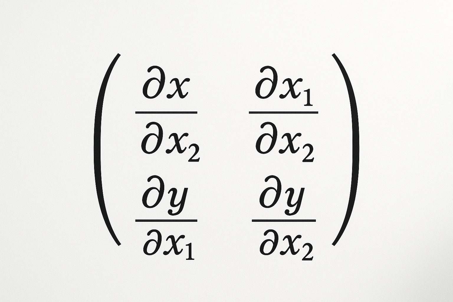
Formally, if you have a differentiable function $\mathbf{f}: \mathbb{R}^2 \to \mathbb{R}^2$ defined by $\mathbf{f}(x,y) = (u(x,y), v(x,y))$, the jacobian matrix 2×2 at a point $(x_0, y_0)$ is:
$$ J = \begin{bmatrix} \frac{\partial u}{\partial x}(x_0,y_0) & \frac{\partial u}{\partial y}(x_0,y_0) \\ \frac{\partial v}{\partial x}(x_0,y_0) & \frac{\partial v}{\partial y}(x_0,y_0) \end{bmatrix} .$$
Each entry tells you the sensitivity of one output component to one input component. Together, they form the best linear approximation to $\mathbf{f}$ near that point. In short, the jacobian matrix 2×2 is the local slope matrix.
“The 2×2 Jacobian is the local derivative of a multi‑input, multi‑output function — it tells you everything about the instantaneous rate of change in every direction.”
Formula and Notation
The jacobian matrix 2×2 is always written with the output partial derivatives in rows and input partials in columns. Standard notation uses $J$ or $D\mathbf{f}$. For the function $\mathbf{f}(x,y) = (u, v)$, we have:
$$ J = \begin{bmatrix} u_x & u_y \\ v_x & v_y \end{bmatrix}, \quad \text{where } u_x = \frac{\partial u}{\partial x}, \; u_y = \frac{\partial u}{\partial y} \dots $$
Notice the order: the first column is derivatives with respect to $x$, the second column with respect to $y$. This convention matches the chain rule and makes matrix multiplication seamless.
How to Compute a Jacobian Matrix 2×2
Computing the jacobian matrix 2×2 is mechanical once you know how to take partial derivatives. Follow these steps:
- Write your function as $\mathbf{f}(x,y) = (u(x,y), v(x,y))$.
- Compute $\frac{\partial u}{\partial x}$ — treat $y$ as constant.
- Compute $\frac{\partial u}{\partial y}$ — treat $x$ as constant.
- Compute $\frac{\partial v}{\partial x}$ and $\frac{\partial v}{\partial y}$ similarly.
- Arrange them in the $2 \times 2$ matrix: top row for $u$, bottom row for $v$.
That’s it! The resulting Jacobian gives you a linear map that approximates the function at that point.
Worked Example: Computing a Jacobian Matrix 2×2
Let’s make it concrete. Consider the function:
$$ \mathbf{f}(x,y) = (x^2 y, \sin(x) + y). $$
Here $u(x,y) = x^2 y$ and $v(x,y) = \sin(x) + y$. We compute the partial derivatives:
- $u_x = \frac{\partial}{\partial x}(x^2 y) = 2xy$
- $u_y = \frac{\partial}{\partial y}(x^2 y) = x^2$
- $v_x = \frac{\partial}{\partial x}(\sin x + y) = \cos x$
- $v_y = \frac{\partial}{\partial y}(\sin x + y) = 1$
The jacobian matrix 2×2 is therefore:
$$ J(x,y) = \begin{bmatrix} 2xy & x^2 \\ \cos x & 1 \end{bmatrix}. $$
At the point $(x,y) = (1, \pi)$, we substitute to get:
$$ J(1,\pi) = \begin{bmatrix} 2\pi & 1 \\ \cos(1) & 1 \end{bmatrix} \approx \begin{bmatrix} 6.283 & 1 \\ 0.540 & 1 \end{bmatrix}. $$
That 2×2 Jacobian now tells us how $\mathbf{f}$ changes near $(1,\pi)$. For small changes $(\Delta x, \Delta y)$, the change in output is approximately $J \cdot (\Delta x, \Delta y)^T$.
🧪 Worked example
For the function $\mathbf{f}(x,y) = (x^2 y, \sin x + y)$:
- Compute partials: $u_x = 2xy$, $u_y = x^2$, $v_x = \cos x$, $v_y = 1$.
- Assemble $J = \begin{bmatrix}2xy & x^2 \\ \cos x & 1\end{bmatrix}$.
- Evaluate at $(1,\pi)$: $J = \begin{bmatrix}2\pi & 1 \\ \cos 1 & 1\end{bmatrix}$.
The resulting Jacobian matrix predicts local change.