Chain Rule for Machine Learning: Essential 2026 Guide

The Chain Rule for Machine Learning is the foundational calculus principle that powers backpropagation in neural networks. If you’ve ever wondered how a model “learns” by adjusting thousands of weights, the answer comes down to this one rule. In this guide, you’ll learn what this principle is, why it’s indispensable, and how to apply it step by step with concrete examples. By the end, you’ll have a deep understanding that will help you debug gradient issues and build better models.

What Is the Chain Rule for Machine Learning?

The Chain Rule for Machine Learning is a formula from calculus for finding the derivative of a composite function. If you have a function $y = f(g(x))$, the derivative $\frac{dy}{dx} = f'(g(x)) \cdot g'(x)$. In plain language: take the derivative of the outer function, plug in the inner function, then multiply by the derivative of the inner function. This rule becomes the workhorse when you have layers of operations — like in a neural network.

Why the Chain Rule for Machine Learning Matters for Neural Networks

Neural networks are built from layers: each layer applies a linear transformation followed by a nonlinear activation. The loss function is a composition of all these layers. To minimize the loss, we need the gradient of the loss with respect to every weight. That’s exactly what this rule computes — but efficiently, layer by layer, from output back to input.

Without the chain rule, training deep networks would be computationally intractable. Backpropagation uses it to reuse intermediate calculations, making gradient computation O(n) instead of O(2^n). This efficiency is what allows models with millions of parameters to be trained in hours.

“The chain rule is not just an abstract calculus concept — it’s the algorithm that makes deep learning practical.”

Step-by-Step: Applying the Chain Rule for Machine Learning

Let’s walk through a concrete example. Suppose we have a simple network with one hidden layer:

$$ z = W_2 \cdot \sigma(W_1 x + b_1) + b_2 $$
where $\sigma$ is the sigmoid activation. Our loss is $L = \frac12 (z – y)^2$. We need $\partial L / \partial W_1$ and $\partial L / \partial W_2$.

Step 1: Identify the composite structure

The chain rule requires that we treat the network as a chain of functions. Write $a = W_1 x + b_1$, $h = \sigma(a)$, $z = W_2 h + b_2$, $L = \frac12(z-y)^2$. Each variable depends on the previous.

Step 2: Compute partial derivatives

This is where the chain rule shines: you can compute each partial derivative independently, then multiply them together. In practice, you’d compute $\partial L / \partial z$ first, then propagate backward. This is exactly what backpropagation does.

For the hidden layer weight $W_1$, the chain includes three intermediate variables. For the output layer weight $W_2$, the chain is shorter: $\partial L / \partial W_2 = (z-y) \cdot h$.

Common Mistakes with the Chain Rule for Machine Learning

A mistake I often see when teaching this rule is forgetting to apply the inner derivative when the outer function itself is composite. For example, if $f(x) = \sin(x^2)$, the derivative is $\cos(x^2) \cdot 2x$, not just $\cos(x^2)$.

Another common error: mixing up the order of multiplication. The chain rule requires multiplying from the outside inward. If you reverse the order, your gradient will be wrong (matrix multiplication is not commutative).

Real-World Use: Backpropagation and Autograd

In modern deep learning frameworks like TensorFlow and PyTorch, the chain rule is implemented via automatic differentiation (autograd). The framework builds a computational graph during the forward pass and then uses the rule to compute gradients during backward pass. Understanding the chain rule helps you interpret those gradients and debug when they vanish or explode.

For example, if you use a sigmoid activation in deep networks, the derivative $\sigma'(x) = \sigma(x)(1-\sigma(x))$ is at most 0.25. Multiplying many such terms via the chain rule leads to vanishing gradients — a key insight you can’t get without knowing the rule.

Mathematical Formulation of the Chain Rule for Machine Learning

Formally, if we have $y = f(u)$ and $u = g(x)$, the Chain Rule for Machine Learning states:

In vector form, if $\mathbf{z} = f(\mathbf{h})$ and $\mathbf{h} = g(\mathbf{x})$, then the Jacobian matrices multiply: $\frac{\partial \mathbf{z}}{\partial \mathbf{x}} = \frac{\partial \mathbf{z}}{\partial \mathbf{h}} \cdot \frac{\partial \mathbf{h}}{\partial \mathbf{x}}$. This is exactly what backpropagation implements.

The chain rule extends to higher dimensions via matrix multiplication. For a neural network with multiple layers, the gradient of the loss $L$ with respect to a weight in layer $k$ is a product of many Jacobians. That’s why understanding the scalar case is the first step.

Advanced: Multivariate Chain Rule for Machine Learning

In practice, neural networks involve multivariate functions. The Chain Rule for Machine Learning then becomes the multivariate chain rule: if $L = L(\mathbf{a})$ and $\mathbf{a} = \mathbf{a}(\mathbf{W})$, then $\frac{\partial L}{\partial \mathbf{W}} = \frac{\partial \mathbf{a}}{\partial \mathbf{W}} \cdot \frac{\partial L}{\partial \mathbf{a}}$. Here, $\frac{\partial \mathbf{a}}{\partial \mathbf{W}}$ is a third-order tensor, but in backpropagation, we use the vectorized form to compute gradients efficiently.

A deep understanding of the multivariate chain rule helps when implementing custom layers or dealing with weight tying. The same principle applies: break the computation into a directed acyclic graph (DAG) and apply the chain rule along each path.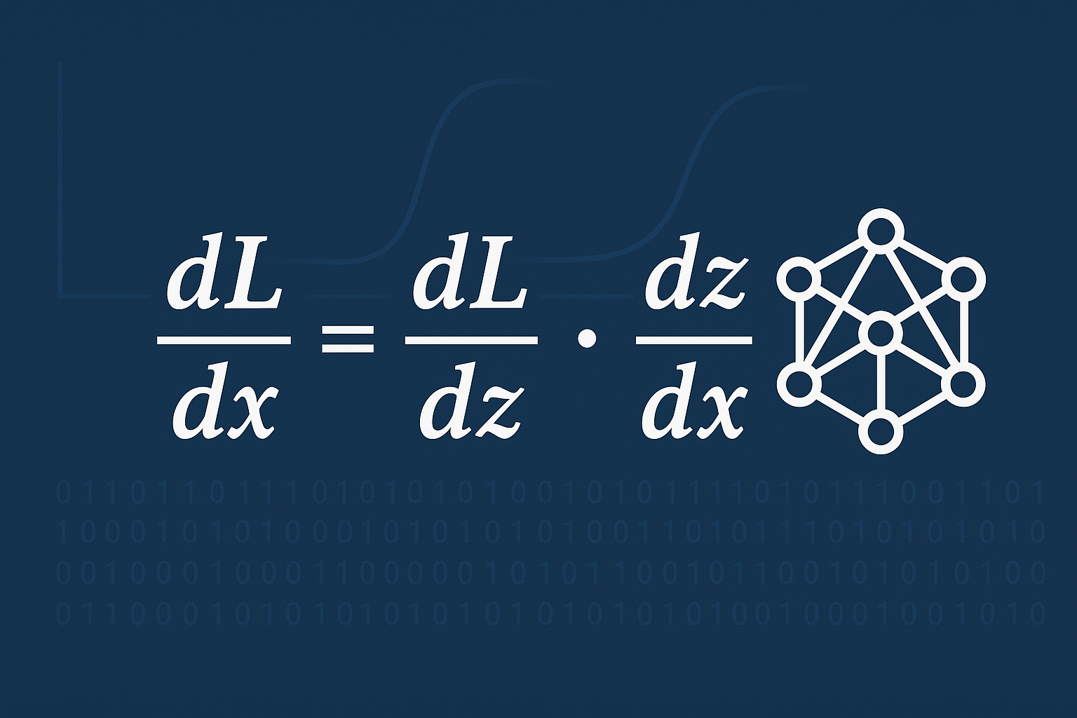

Related Calculus Concepts for ML

The chain rule is one of several calculus tools you’ll use. For example, the derivative of a fraction (also known as the quotient rule) is useful when dealing with normalization layers. Check out our companion guide on the Derivative of a Fraction: A Visual and Practical Guide to the Quotient Rule for detailed examples.

You also need to understand limits to grasp the definition of a derivative. See 8 Core Properties of Limits with Step-by-Step Examples for Beginners for a solid foundation. And if you’re working with vectors (common in neural network inputs), Sum of Vectors: The Essential 2026 Guide to Vector Addition will help.

Applying the Chain Rule for Machine Learning in Code

You don’t need to manually apply the chain rule every time — libraries like PyTorch do it for you. But knowing what’s under the hood makes you a better engineer. For instance, when you call loss.backward(), PyTorch traverses the computational graph and applies the rule to compute gradients. If you understand the chain rule, you can anticipate gradient flow issues and adjust your architecture.

Here’s a simple PyTorch example:

import torch
x = torch.tensor([1.0, 2.0], requires_grad=True)
w = torch.tensor([2.0, -1.0], requires_grad=True)
b = torch.tensor([0.5], requires_grad=True)
z = torch.dot(w, x) + b   # linear layer
loss = z.sum()  # simple loss
loss.backward()
print(w.grad)  # gradient computed via chain rule

In this snippet, backward() uses the chain rule to compute $\partial \text{loss} / \partial w = x$, $\partial \text{loss} / \partial b = 1$, and $\partial \text{loss} / \partial x = w$. You can verify this manually.

Master the Chain Rule for Machine Learning

The Chain Rule for Machine Learning is not optional knowledge for a deep learning practitioner. It’s the key that unlocks gradient-based learning. Whether you’re tuning a learning rate or designing a new architecture, the rule is always at work. Start with the scalar version, then extend to vectors and matrices. Practice with simple networks until the pattern becomes second nature.

If you want to go deeper, explore how the chain rule interacts with matrix multiplication. Our guide on The Ultimate Guide to the Row by Column Method: 5 Essential Rules for Matrix Multiplication will help you compute Jacobians efficiently. Also, review the Identity Matrix: Definition, Properties, and Examples (2026) for understanding derivative of linear transformations.

The chain rule is the bridge from calculus to code. Master it, and you’ll have a powerful intuition for how neural networks learn.

Frequently Asked Questions

▶ Watch related videos on YouTube: Chain Rule for Machine Learning video tutorials *This article contains affiliate links. We may earn a commission if you click through and make a purchase, at no extra cost to you. However, our recommendations are independent and based on thorough research.*

• Essential Unit Vectors: 7 Key Concepts for Machine Learning

• 7 Essential Types of Vectors for ML Practitioners

• Linear Algebra For Machine Learning: 6 Essential Concepts & Tools

• 2×2 Identity Matrix: 9 Essential Properties (2026 Guide)

• Linearly Independent Vectors: Essential Guide (2026)

• 3 by 3 Matrix: The Essential 2026 Guide to Determinant, Inverse & More

• The Ultimate Dot Product Guide: 10 Essential Rules for Beginners in 2026

• Linear Dependence of Vectors: The Complete Guide to Understanding Vector Relationships in Machine Learning