This logistic regression example walks through a complete classification problem from raw data to a final prediction, using the friendliest dataset in machine learning: hours studied versus whether a student passes an exam. By the end you will be able to plug a number into the sigmoid by hand, read off a probability, and classify it — the whole pipeline in one worked logistic regression example.
The setup for our logistic regression example
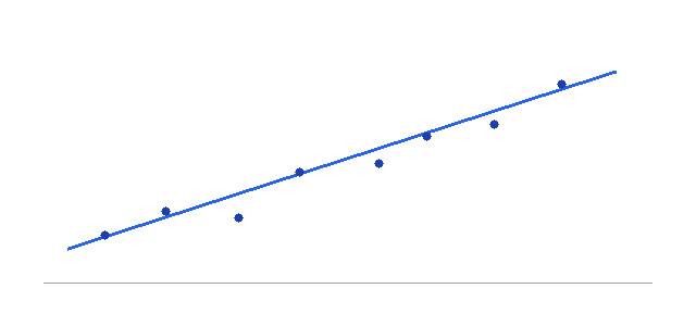
Imagine you collected data on a handful of students: how many hours each studied ($x$) and whether they passed the exam ($y$, coded as $1$ for pass and $0$ for fail). The target is a yes/no outcome, so this is a classification task — exactly what logistic regression is built for. Our goal is to learn a model that, given hours studied, returns the probability of passing and then a clean pass/fail decision.
Logistic regression assumes the log-odds of passing is a straight line in $x$, and it produces a probability through the sigmoid (logistic) function:
$$p = \frac{1}{1 + e^{-(\beta_0 + \beta_1 x)}}, \qquad z = \beta_0 + \beta_1 x$$Here $z$ is the linear part (the log-odds) and $p$ is the probability after the sigmoid squeezes $z$ into the range $(0,1)$.
Logistic regression example: step by step
With the fitted coefficients in hand, every prediction is just arithmetic. Here is the worked logistic regression example, step by step, for a student who studied 2 hours and another who studied 4 hours.
- Write down the model. Using the fitted values, $z = \beta_0 + \beta_1 x = -4.0777 + 1.5046\,x$, and $p = \dfrac{1}{1 + e^{-z}}$. Every prediction below reuses these two lines.
- Predict for $x = 2$ hours — compute $z$. Substitute: $z = -4.0777 + 1.5046 \times 2 = -4.0777 + 3.0092 = -1.0685$. The log-odds are negative, which already hints the probability will be below one half.
- Turn $z$ into a probability. Apply the sigmoid: $p = \dfrac{1}{1 + e^{-(-1.0685)}} = \dfrac{1}{1 + e^{1.0685}} = \dfrac{1}{1 + 2.911} \approx 0.256$. So a 2-hour student has about a 25.6% chance of passing.
- Predict for $x = 4$ hours — compute $z$. Substitute again: $z = -4.0777 + 1.5046 \times 4 = -4.0777 + 6.0184 = 1.9407$. This time the log-odds are positive.
- Turn that $z$ into a probability. $p = \dfrac{1}{1 + e^{-1.9407}} = \dfrac{1}{1 + 0.1437} \approx 0.874$. A 4-hour student has about an 87.4% chance of passing — a dramatic jump from just two extra hours.
- Classify with a threshold. The default rule is predict pass when $p \ge 0.5$. The 2-hour student ($p \approx 0.256$) is classified as fail; the 4-hour student ($p \approx 0.874$) is classified as pass.
Interpreting the coefficients in this example
The slope $\beta_1 = 1.5046$ is the increase in log-odds of passing per extra hour studied. Log-odds are hard to feel intuitively, so we exponentiate to get the odds ratio:
$$e^{\beta_1} = e^{1.5046} \approx 4.5$$That number is the headline of the whole logistic regression example: each additional hour of study multiplies the odds of passing by about 4.5. If a student currently has 1-to-1 odds (a coin flip), one more hour pushes the odds to roughly 4.5-to-1 in favor of passing. The intercept $\beta_0 = -4.0777$ is the log-odds for a student who studies zero hours — deeply negative, meaning passing without studying is very unlikely under this model. For more on reading these numbers, see our guide on odds ratio interpretation.
Finding the decision boundary
The decision boundary is the value of $x$ where the model is perfectly undecided — where $p = 0.5$, equivalently $z = 0$. Solving $\beta_0 + \beta_1 x = 0$ gives:
$$x = -\frac{\beta_0}{\beta_1} = -\frac{-4.0777}{1.5046} \approx 2.71 \text{ hours}$$So the tipping point is about 2.71 hours of study. Below it the model predicts fail; above it, pass. Notice the 2-hour student sits just below the boundary (predicted fail) and the 4-hour student sits well above it (predicted pass) — consistent with the probabilities we computed.
The full prediction table
To see the S-shaped sigmoid in action, here is the same logistic regression example evaluated across a range of study hours. Each row reuses $z = -4.0777 + 1.5046\,x$ and $p = 1/(1+e^{-z})$:
| Hours $x$ | $z = \beta_0 + \beta_1 x$ | Probability $p$ | Predicted class |
|---|---|---|---|
| 1 | $-2.5731$ | $0.071$ | Fail (0) |
| 2 | $-1.0685$ | $0.256$ | Fail (0) |
| 2.71 | $\approx 0.000$ | $0.500$ | Boundary |
| 3 | $0.4361$ | $0.607$ | Pass (1) |
| 4 | $1.9407$ | $0.874$ | Pass (1) |
| 5 | $3.4453$ | $0.969$ | Pass (1) |
Watch the probability climb smoothly from $0.071$ toward $0.969$ as hours increase — that gentle S-curve, never dipping below 0 or rising above 1, is the signature of logistic regression. The class flips from fail to pass right as $x$ crosses the 2.71-hour boundary.
🤖 ML context
This logistic regression example is the gateway to classification across machine learning. The very same sigmoid-on-a-linear-term is a single neuron, so mastering this is your first step into neural networks. To see how it differs from predicting numbers, compare it with logistic regression vs linear regression, and deepen your reading of the slope with odds ratio interpretation. Build live intuition with the logistic regression calculator.
Frequently asked questions
What is a simple logistic regression example?
How do you calculate probability in logistic regression?
What does the logistic regression coefficient mean?
How do you find the decision boundary?
How do you classify a prediction in logistic regression?
Key takeaways
This logistic regression example showed the full pipeline: fit coefficients by maximum likelihood ($\beta_0 = -4.0777$, $\beta_1 = 1.5046$), compute $z = \beta_0 + \beta_1 x$, push it through the sigmoid to get a probability, classify with a 0.5 threshold, read the odds ratio $e^{\beta_1} \approx 4.5$, and locate the 2.71-hour decision boundary. Continue with the logistic regression calculator, the logistic regression vs linear regression comparison, the guide to odds ratio interpretation, or the formal reference on Wikipedia.